EasyVVUQ - Basic Concepts

Author: Vytautas Jancauskas, LRZ (jancauskas@lrz.de)

If this is your first Jupyter Notebook - you can execute code cells by selecting them and pressing Shift+Enter. Just have in mind that the order of execution might matter (if later cells depend on things done in earlier ones).

This tutorial shows a simple EasyVVUQ workflow in action. The example used here is a simulation of a vertical deflection of a tube. The model is that of a round metal tube suspended on each end and force being applied at a certain point along it’s length. The model measures how large is the deflection at the point force is applied. Full description of it can be found here. This model was chosen since it is intuitively easy to understand even without any background in the relative field. It is also easy to interpret the results. We will use EasyVVUQ to determine the influence each of the input parameters has on the vertical deflection at point a.

The usage of the application is:

beam <input_file>

It outputs a single file called output.json, which will look like {'g1': x, 'g2': y, 'g3': y} where g1 is the vertical displacement at point a and g2, g3 are displaced angles of the tube at the left and right ends respectively.

The beam.template is a template input file, in JSON format

{"outfile": "$outfile", "F": $F, "L": $L, "a": $a, "D": $D, "d": $d, "E": $E}

The values for each key are tags (signified by the $ delimiter) which will be substituted by EasyVVUQ with values to sample the parameter space. In the following tutorial, the template will be used to generate files called input.json that will be the input to each run of beam.

So, for example (commands preceded by an exclamation mark are treated as shell commands):

!echo "{\"outfile\": \"output.json\", \"F\": 1.0, \"L\": 1.5, \"a\": 1.0, \"D\": 0.8, \"d\": 0.1, \"E\": 200000}" > input.json

!./beam input.json

!cat output.json

In this tutorial we will see how to use EasyVVUQ to do variance based sensitivity analysis using stochastic collocation. It is one of several methods that EasyVVUQ supports for this purpose (others being Monte Carlo and Polynomial Chaos Expansion methods). While stochastic collocation supports more complicated scenarios we only explore the basic functionality.

Campaign

We need to import EasyVVUQ as well as ChaosPy (we use it’s distributions) and matplotlib for plotting later on.

import easyvvuq as uq
import chaospy as cp
import matplotlib.pyplot as plt

We will describe the parameters. This is done for validation purposes (so that input parameters outside valid ranges given an error. Also this is where you can specify default values for input parameters that you don’t want to vary in the analysis. Only the type and the default value fields are mandatory.

params = {
    "F": {"type": "float", "default": 1.0},
    "L": {"type": "float", "default": 1.5},
    "a": {"type": "float", "min": 0.7, "max": 1.2, "default": 1.0},
    "D": {"type": "float", "min": 0.75, "max": 0.85, "default": 0.8},
    "d": {"type": "float", "default": 0.1},
    "E": {"type": "float", "default": 200000},
    "outfile": {"type": "string", "default": "output.json"}
}

Next step is to specify how the input files for the simulation are to be created and how EasyVVUQ is to parse the output of the simulation. This is the job of the Encoder and Decoder classes. Our simulation takes a very simple JSON file as input. So we can just use the GenericEncoder which is a template based encoder. It will replace all keys in the template file with respective values. In this case they are identified by the $ that precedes them. Alternatively, there are more complex encoders based on, for example, the Jinja2 templating language. Encoders can also do more complicated things, such as prepare a directory structure if your simulation requires such. If it requires several input files you can use a multiencoder to combine several encoders, each of which responsible for a single input file. They can also be used to copy files over to the run directory.

Decoder is responsible for parsing the otuput of the simulation. We use the JSONDecoder to extract the needed value. There also exist ready made decoders for YAML and CSV. You can also easily write your own by inheriting from the BaseDecoder class.

encoder = uq.encoders.GenericEncoder(template_fname='beam.template', delimiter='$', target_filename='input.json')
decoder = uq.decoders.JSONDecoder(target_filename='output.json', output_columns=['g1'])

Campaign is the central hub in which operations take place. It is responsible for running your simulations, gathering the results, storing them in the Database, retrieving them for analysis, etc. The Campaign in EasyVVUQ is very powerful and supports multiple applications, sampling, analysis and execution methods. It also lets you save progress and retrieve results later for analysis. Here we only look at a simple case.

campaign = uq.Campaign(name='beam', params=params, encoder=encoder, decoder=decoder)

First we need to define the input parameter distributions. We have chosen 4 of the 6 available inputs. This is partly because this means that we won’t have to sample at too many points and partly because I’ve found that these influence the output variable the most.

vary = {
    "F": cp.Normal(1, 0.1),
    "L": cp.Normal(1.5, 0.01),
    "a": cp.Uniform(0.7, 1.2),
    "D": cp.Triangle(0.75, 0.8, 0.85)
}

We have to choose the sampler next. For this task we can use either Stochastic Collocation, Polynomial Chaos Expansion or QMC samplers. Stochastic Collocation is fast for this problem size so that is what we chose.

campaign.set_sampler(uq.sampling.SCSampler(vary=vary, polynomial_order=3))

For this tutorial we have chosen to run the simulation on the local machine. This will done in parallel with up to 8 tasks running concurrently. Alternatives are execution in the Cloud (via the ExecuteKubernetes action) or on HPC machines.

execution = campaign.sample_and_apply(action=uq.actions.ExecuteLocalV2("beam input.json"), batch_size=8).start()

The execution can take a bit since we need to generate several hundred samples. We asked it to evaluate 8 samples in parallel. You can track progress by using the progress method. You can also check progress automatically and resume execution after it is done if you want to run this inside a script rather than interactively.

execution.progress()

{'ready': 188, 'active': 8, 'finished': 60, 'failed': 0}

We then call the analyse method whose functionality will depend on the sampling method used. It returns an `AnalysisResults <>`__ object which can be used to retrieve numerical values or plot the results. In this case Sobols indices.

results = campaign.analyse(qoi_cols=['g1'])

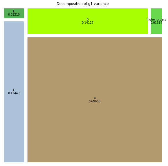
We can plot the results in a treemap format. Each square representing the relative influence of that parameter to the variance of the output variable (vertical displacement at point a). A square labeled higher orders represent the influence of the interactions between the input parameters.

results.plot_sobols_treemap('g1', figsize=(10, 10))
plt.axis('off');

Alternatively you can get the Sobol index values using the method call below.

results.sobols_first()