EasyVVUQ - Jinja encoder tutorial

This is a small modification of the basic tutorial on the simple beam model. In particular, will show how to use mathmatical expressions inside a Jinja template. For more information in encoding and decoding see the tutorials/encoder_decoder_tutorial.ipynb notebook.

Campaign

We need to import EasyVVUQ as well as ChaosPy (we use it’s distributions) and matplotlib for plotting later on.

import os
import easyvvuq as uq
import chaospy as cp
import matplotlib.pyplot as plt
from easyvvuq.actions import CreateRunDirectory, Encode, Decode, CleanUp, ExecuteLocal, Actions

/Volumes/UserData/dpc/GIT/EasyVVUQ/env_3.12/lib/python3.12/site-packages/chaospy/__init__.py:9: UserWarning: pkg_resources is deprecated as an API. See https://setuptools.pypa.io/en/latest/pkg_resources.html. The pkg_resources package is slated for removal as early as 2025-11-30. Refrain from using this package or pin to Setuptools<81.
  import pkg_resources

We will describe the parameters. This is done for validation purposes (so that input parameters outside valid ranges given an error. Also this is where you can specify default values for input parameters that you don’t want to vary in the analysis. Only the type and the default value fields are mandatory.

params = {
    "F": {"type": "float", "default": 1.0},
    "L": {"type": "float", "default": 1.5},
    "a": {"type": "float", "min": 0.7, "max": 1.2, "default": 1.0},
    "D": {"type": "float", "min": 0.75, "max": 0.85, "default": 0.8},
    "d": {"type": "float", "default": 0.1},
    "E": {"type": "float", "default": 200000},
    "power" : {"type": "float", "default": 0.5},
    "outfile": {"type": "string", "default": "output.json"}
}

Jinja encoder

Below we find the only deviation from the basic tutorial, namely the use of the Jinja decoder with a mathmatical expression for the a variable. The standard Jinja template would look like:

{"outfile": "{{outfile}}",
"F": {{F}},
"L": {{L}},
"a": {{a}},
"D": {{D}},
"d": {{d}},
"E": {{E}}
}

This is replaces every {{variable}} with a numeric value. If that the variable appears in the vary, the value will be drawn from the specified probability distribution. If it does not appear in vary, the default value as specified in the params dict will be used. The result will be a JSON file that is read by the beam model. It does not have to be a JSON file, this same principle will hold for any type of template file.

The Jinja encoder is flexible in the sense that mathematical expressions can also be used. As an example, consider the followin template:

{"outfile": "{{outfile}}",
"F": {{F}},
"L": {{L}},
"a": {{a ** power}},
"D": {{D}},
"d": {{d}},
"E": {{E}}
}

This is the same as before, except now the square root of a is taken. Here, power is also defined in the params dict. Since power is not in vary, the value of 0.5 is always used.

encoder = uq.encoders.JinjaEncoder(template_fname='beam.jinja', target_filename='input.json')

The rest of this turorial proceeds unmodified from the basic tutorial.

decoder = uq.decoders.JSONDecoder(target_filename='output.json', output_columns=['g1'])
execute = ExecuteLocal('{}/beam input.json'.format(os.getcwd()))

actions = Actions(CreateRunDirectory('/tmp', flatten=True),
                  Encode(encoder), execute, Decode(decoder))

Campaign is the central hub in which operations take place. It is responsible for running your simulations, gathering the results, storing them in the Database, retrieving them for analysis, etc. The Campaign in EasyVVUQ is very powerful and supports multiple applications, sampling, analysis and execution methods. It also lets you save progress and retrieve results later for analysis. Here we only look at a simple case.

campaign = uq.Campaign(name='beam', params=params, actions=actions, work_dir='/tmp')

/Volumes/UserData/dpc/GIT/EasyVVUQ/env_3.12/lib/python3.12/site-packages/cerberus/validator.py:618: UserWarning: These types are defined both with a method and in the'types_mapping' property of this validator: {'integer'}
  warn(
/Volumes/UserData/dpc/GIT/EasyVVUQ/env_3.12/lib/python3.12/site-packages/cerberus/validator.py:618: UserWarning: These types are defined both with a method and in the'types_mapping' property of this validator: {'integer'}
  warn(

First we need to define the input parameter distributions. We have chosen 4 of the 6 available inputs. This is partly because this means that we won’t have to sample at too many points and partly because I’ve found that these influence the output variable the most.

vary = {
    "F": cp.Normal(1, 0.1),
    "L": cp.Normal(1.5, 0.01),
    "a": cp.Uniform(0.7, 1.2),
    "D": cp.Triangle(0.75, 0.8, 0.85)
}

We have to choose the sampler next. For this task we can use either Stochastic Collocation, Polynomial Chaos Expansion or QMC samplers. Stochastic Collocation is fast for this problem size so that is what we chose.

campaign.set_sampler(uq.sampling.PCESampler(vary=vary, polynomial_order=1))

For this tutorial we have chosen to run the simulation on the local machine. This will done in parallel with up to 8 tasks running concurrently. Alternatives are execution in the Cloud (via the ExecuteKubernetes action) or on HPC machines.

campaign.execute().collate()

The execution can take a bit since we need to generate several hundred samples. We asked it to evaluate 8 samples in parallel. You can track progress by using the progress method. You can also check progress automatically and resume execution after it is done if you want to run this inside a script rather than interactively.

campaign.get_collation_result()

	run_id	iteration	F	L	a	D	d	E	power	outfile	g1
	0	0	0	0	0	0	0	0	0	0	0
0	1	0	0.9	1.49	0.805662	0.779588	0.1	200000	0.5	output.json	-0.000008
1	2	0	0.9	1.49	0.805662	0.820412	0.1	200000	0.5	output.json	-0.000006
2	3	0	0.9	1.49	1.094338	0.779588	0.1	200000	0.5	output.json	-0.000006
3	4	0	0.9	1.49	1.094338	0.820412	0.1	200000	0.5	output.json	-0.000005
4	5	0	0.9	1.51	0.805662	0.779588	0.1	200000	0.5	output.json	-0.000008
5	6	0	0.9	1.51	0.805662	0.820412	0.1	200000	0.5	output.json	-0.000007
6	7	0	0.9	1.51	1.094338	0.779588	0.1	200000	0.5	output.json	-0.000006
7	8	0	0.9	1.51	1.094338	0.820412	0.1	200000	0.5	output.json	-0.000005
8	9	0	1.1	1.49	0.805662	0.779588	0.1	200000	0.5	output.json	-0.000010
9	10	0	1.1	1.49	0.805662	0.820412	0.1	200000	0.5	output.json	-0.000008
10	11	0	1.1	1.49	1.094338	0.779588	0.1	200000	0.5	output.json	-0.000007
11	12	0	1.1	1.49	1.094338	0.820412	0.1	200000	0.5	output.json	-0.000006
12	13	0	1.1	1.51	0.805662	0.779588	0.1	200000	0.5	output.json	-0.000010
13	14	0	1.1	1.51	0.805662	0.820412	0.1	200000	0.5	output.json	-0.000008
14	15	0	1.1	1.51	1.094338	0.779588	0.1	200000	0.5	output.json	-0.000008
15	16	0	1.1	1.51	1.094338	0.820412	0.1	200000	0.5	output.json	-0.000006

We then call the analyse method whose functionality will depend on the sampling method used. It returns an `AnalysisResults <>`__ object which can be used to retrieve numerical values or plot the results. In this case Sobols indices.

results = campaign.analyse(qoi_cols=['g1'])

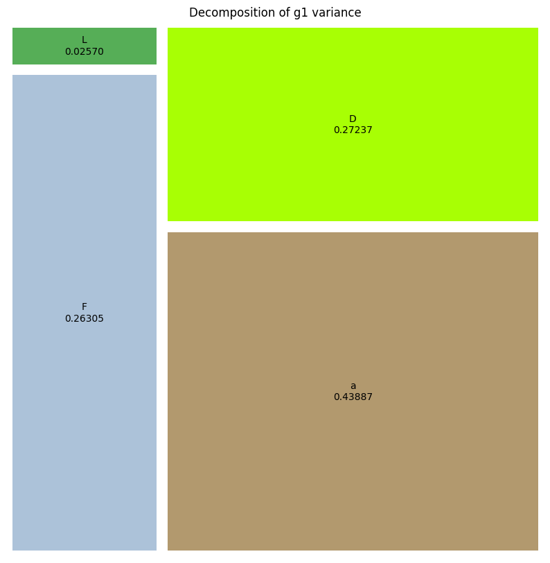
We can plot the results in a treemap format. Each square representing the relative influence of that parameter to the variance of the output variable (vertical displacement at point a). A square labeled higher orders represent the influence of the interactions between the input parameters.

results.plot_sobols_treemap('g1', figsize=(10, 10))
plt.axis('off');

/Volumes/UserData/dpc/GIT/EasyVVUQ/env_3.12/lib/python3.12/site-packages/easyvvuq/analysis/results.py:467: UserWarning: FigureCanvasAgg is non-interactive, and thus cannot be shown
  fig.show()

Alternatively you can get the Sobol index values using the method call below.

results.sobols_first('g1')

{'F': array([0.26305477]),
 'L': array([0.02570021]),
 'a': array([0.43887154]),
 'D': array([0.27237348])}

results.supported_stats()

['min', 'max', '10%', '90%', '1%', '99%', 'median', 'mean', 'var', 'std']

results._get_sobols_first('g1', 'F')

array([0.26305477])

results.sobols_total('g1', 'F')

array([0.26305477])