Sensitivity analysis for the Ishigama function using PCE
Run an EasyVVUQ campaign to analyze the sensitivity for the Ishigami function
This is done with PCE.
[1]:
# Run an EasyVVUQ campaign to analyze the sensitivity for the Ishigami function
# This is done with PCE.
%matplotlib inline
import os
import easyvvuq as uq
import chaospy as cp
import pickle
import numpy as np
import matplotlib.pylab as plt
import time
import pandas as pd
[2]:
np.__version__
[2]:
'1.26.4'
[3]:
# Define the Ishigami function
def ishigamiSA(a,b):
    '''Exact sensitivity indices of the Ishigami function for given a and b.
    From https://openturns.github.io/openturns/master/examples/meta_modeling/chaos_ishigami.html
    '''
    var = 1.0/2 + a**2/8 + b*np.pi**4/5 + b**2*np.pi**8/18
    S1 = (1.0/2 + b*np.pi**4/5+b**2*np.pi**8/50)/var
    S2 = (a**2/8)/var
    S3 = 0
    S13 = b**2*np.pi**8/2*(1.0/9-1.0/25)/var
    exact = {
            'expectation' : a/2,
            'variance' : var,
            'S1' : (1.0/2 + b*np.pi**4/5+b**2*np.pi**8.0/50)/var,
            'S2' : (a**2/8)/var,
            'S3' : 0,
            'S12' : 0,
            'S23' : 0,
            'S13' : S13,
            'S123' : 0,
            'ST1' : S1 + S13,
            'ST2' : S2,
            'ST3' : S3 + S13
            }
    return exact

Ishigami_a = 7.0
Ishigami_b = 0.1
exact = ishigamiSA(Ishigami_a, Ishigami_b)
[4]:
# define a model to run the Ishigami code directly from python, expecting a dictionary and returning a dictionary
def run_ishigami_model(input):
    import Ishigami
    qois = ["Ishigami"]
    del input['out_file']
    return {qois[0]: Ishigami.evaluate(**input)}
[5]:
# Define parameter space
def define_params():
    return {
        "x1":       {"type": "float",   "min": -np.pi,     "max": np.pi,      "default": 0.0},
        "x2":       {"type": "float",   "min": -np.pi,     "max": np.pi,      "default": 0.0},
        "x3":       {"type": "float",   "min": -np.pi,     "max": np.pi,      "default": 0.0},
        "a":        {"type": "float",   "min": Ishigami_a, "max": Ishigami_a, "default": Ishigami_a},
        "b":        {"type": "float",   "min": Ishigami_b, "max": Ishigami_b, "default": Ishigami_b},
        "out_file": {"type": "string",  "default": "output.csv"}
    }
[6]:
# Define parameter space
def define_vary():
    return {
        "x1":   cp.Uniform(-np.pi, np.pi),
        "x2":   cp.Uniform(-np.pi, np.pi),
        "x3":   cp.Uniform(-np.pi, np.pi)
    }
[7]:
# Set up and run a campaign
def run_campaign(pce_order=2, use_files=False):

    times = np.zeros(7)

    time_start = time.time()
    time_start_whole = time_start

    # Set up a fresh campaign called "Ishigami_pce."
    my_campaign = uq.Campaign(name='Ishigami_pce.')

    # Create an encoder and decoder for PCE test app
    if use_files:
        encoder = uq.encoders.GenericEncoder(template_fname='Ishigami.template',
                                             delimiter='$',
                                             target_filename='Ishigami_in.json')

        decoder = uq.decoders.SimpleCSV(target_filename="output.csv",
                                        output_columns=["Ishigami"])

        execute = uq.actions.ExecuteLocal('python3 %s/Ishigami.py Ishigami_in.json' % (os.getcwd()))

        actions = uq.actions.Actions(uq.actions.CreateRunDirectory('/tmp'),
                          uq.actions.Encode(encoder), execute, uq.actions.Decode(decoder))
    else:
        actions = uq.actions.Actions(uq.actions.ExecutePython(run_ishigami_model))

    # Add the app (automatically set as current app)
    my_campaign.add_app(name="Ishigami", params=define_params(), actions=actions)

    # Create the sampler
    time_end = time.time()
    times[1] = time_end-time_start
    print('Time for phase 1 = %.3f' % (times[1]))

    time_start = time.time()
    # Associate a sampler with the campaign
    my_campaign.set_sampler(uq.sampling.PCESampler(vary=define_vary(), polynomial_order=pce_order))

    # Will draw all (of the finite set of samples)
    my_campaign.draw_samples()
    print('Number of samples = %s' % my_campaign.get_active_sampler().count)

    time_end = time.time()
    times[2] = time_end-time_start
    print('Time for phase 2 = %.3f' % (times[2]))

    time_start = time.time()
    # Run the cases
    my_campaign.execute(sequential=True).collate(progress_bar=True)

    time_end = time.time()
    times[3] = time_end-time_start
    print('Time for phase 3 = %.3f' % (times[3]))

    time_start = time.time()
    # Get the results
    results_df = my_campaign.get_collation_result()

    time_end = time.time()
    times[4] = time_end-time_start
    print('Time for phase 4 = %.3f' % (times[4]))

    time_start = time.time()
    # Post-processing analysis
    results = my_campaign.analyse(qoi_cols=["Ishigami"])

    time_end = time.time()
    times[5] = time_end-time_start
    print('Time for phase 5 = %.3f' % (times[5]))

    time_start = time.time()
    # Save the results
    pickle.dump(results, open('Ishigami_results.pickle','bw'))
    time_end = time.time()
    times[6] = time_end-time_start
    print('Time for phase 6 = %.3f' % (times[6]))

    times[0] = time_end - time_start_whole

    return results_df, results, times, pce_order, my_campaign.get_active_sampler().count
[8]:
# Calculate the polynomial chaos expansion for a range of orders

R = {}
for pce_order in range(1, 21):
    R[pce_order] = {}
    (R[pce_order]['results_df'],
     R[pce_order]['results'],
     R[pce_order]['times'],
     R[pce_order]['order'],
     R[pce_order]['number_of_samples']) = run_campaign(pce_order=pce_order, use_files=False)
Time for phase 1 = 0.035
Number of samples = 8
Time for phase 2 = 0.042
100%|███████████████████████████████████████████| 8/8 [00:00<00:00, 2215.40it/s]
Traceback (most recent call last):
  File "/Volumes/UserData/dpc/GIT/EasyVVUQ/env_3.12/lib/python3.12/site-packages/easyvvuq/analysis/pce_analysis.py", line 495, in analyse
    dY_hat = build_surrogate_der(fit, verbose=False)
             ^^^^^^^^^^^^^^^^^^^^^^^^^^^^^^^^^^^^^^^
  File "/Volumes/UserData/dpc/GIT/EasyVVUQ/env_3.12/lib/python3.12/site-packages/easyvvuq/analysis/pce_analysis.py", line 347, in build_surrogate_der
    assert(sum(sum(np.array(Y_hat[t].exponents))) == 0)
           ^^^^^^^^^^^^^^^^^^^^^^^^^^^^^^^^^^^^^^^^^^^
AssertionError
Time for phase 3 = 0.023
Time for phase 4 = 0.003
Time for phase 5 = 0.031
Time for phase 6 = 0.002
Time for phase 1 = 0.010
Number of samples = 27
Time for phase 2 = 0.059
100%|█████████████████████████████████████████| 27/27 [00:00<00:00, 5205.29it/s]
Time for phase 3 = 0.010
Time for phase 4 = 0.002
Time for phase 5 = 0.102
Time for phase 6 = 0.001
Time for phase 1 = 0.006
Number of samples = 64
Time for phase 2 = 0.091
100%|█████████████████████████████████████████| 64/64 [00:00<00:00, 5930.44it/s]
Time for phase 3 = 0.016
Time for phase 4 = 0.002
Time for phase 5 = 0.167
Time for phase 6 = 0.001
Time for phase 1 = 0.006
Number of samples = 125
Time for phase 2 = 0.147
100%|███████████████████████████████████████| 125/125 [00:00<00:00, 6213.12it/s]
Time for phase 3 = 0.027
Time for phase 4 = 0.003
Time for phase 5 = 0.305
Time for phase 6 = 0.001
Time for phase 1 = 0.006
Number of samples = 216
Time for phase 2 = 0.192
100%|███████████████████████████████████████| 216/216 [00:00<00:00, 6028.10it/s]
Time for phase 3 = 0.046
Time for phase 4 = 0.006
Time for phase 5 = 0.485
Time for phase 6 = 0.001
Time for phase 1 = 0.006
Number of samples = 343
Time for phase 2 = 0.240
100%|███████████████████████████████████████| 343/343 [00:00<00:00, 2419.45it/s]
Time for phase 3 = 0.154
Time for phase 4 = 0.006
Time for phase 5 = 0.766
Time for phase 6 = 0.001
Time for phase 1 = 0.006
Number of samples = 512
Time for phase 2 = 0.319
100%|███████████████████████████████████████| 512/512 [00:00<00:00, 6729.86it/s]
Time for phase 3 = 0.093
Time for phase 4 = 0.007
Time for phase 5 = 1.293
Time for phase 6 = 0.004
Time for phase 1 = 0.007
Number of samples = 729
Time for phase 2 = 0.414
100%|███████████████████████████████████████| 729/729 [00:00<00:00, 6692.38it/s]
Time for phase 3 = 0.131
Time for phase 4 = 0.009
Time for phase 5 = 2.202
Time for phase 6 = 0.001
Time for phase 1 = 0.007
Number of samples = 1000
Time for phase 2 = 0.561
100%|█████████████████████████████████████| 1000/1000 [00:00<00:00, 6859.50it/s]
Time for phase 3 = 0.172
Time for phase 4 = 0.011
Time for phase 5 = 3.796
Time for phase 6 = 0.002
Time for phase 1 = 0.025
Number of samples = 1331
Time for phase 2 = 0.813
100%|█████████████████████████████████████| 1331/1331 [00:00<00:00, 6505.47it/s]
Time for phase 3 = 0.240
Time for phase 4 = 0.015
Time for phase 5 = 6.412
Time for phase 6 = 0.002
Time for phase 1 = 0.008
Number of samples = 1728
Time for phase 2 = 0.850
100%|█████████████████████████████████████| 1728/1728 [00:00<00:00, 6791.62it/s]
Time for phase 3 = 0.299
Time for phase 4 = 0.094
Time for phase 5 = 10.218
Time for phase 6 = 0.009
Time for phase 1 = 0.015
Number of samples = 2197
Time for phase 2 = 1.097
100%|█████████████████████████████████████| 2197/2197 [00:00<00:00, 6577.30it/s]
Time for phase 3 = 0.396
Time for phase 4 = 0.140
Time for phase 5 = 17.613
Time for phase 6 = 0.016
Time for phase 1 = 0.011
Number of samples = 2744
Time for phase 2 = 1.335
100%|█████████████████████████████████████| 2744/2744 [00:00<00:00, 6627.28it/s]
Time for phase 3 = 0.602
Time for phase 4 = 0.028
Time for phase 5 = 25.524
Time for phase 6 = 0.012
Time for phase 1 = 0.022
Number of samples = 3375
Time for phase 2 = 1.766
100%|█████████████████████████████████████| 3375/3375 [00:00<00:00, 6642.32it/s]
Time for phase 3 = 0.594
Time for phase 4 = 0.099
Time for phase 5 = 38.722
Time for phase 6 = 0.005
Time for phase 1 = 0.014
Number of samples = 4096
Time for phase 2 = 2.180
100%|█████████████████████████████████████| 4096/4096 [00:00<00:00, 6635.85it/s]
Time for phase 3 = 0.727
Time for phase 4 = 0.043
Time for phase 5 = 58.738
Time for phase 6 = 0.006
Time for phase 1 = 0.012
Number of samples = 4913
Time for phase 2 = 2.675
100%|█████████████████████████████████████| 4913/4913 [00:00<00:00, 6714.53it/s]
Time for phase 3 = 0.942
Time for phase 4 = 0.047
Time for phase 5 = 85.127
Time for phase 6 = 0.005
Time for phase 1 = 0.018
Number of samples = 5832
Time for phase 2 = 3.358
100%|█████████████████████████████████████| 5832/5832 [00:00<00:00, 6390.76it/s]
Time for phase 3 = 1.097
Time for phase 4 = 0.133
Time for phase 5 = 121.527
Time for phase 6 = 0.007
Time for phase 1 = 0.013
Number of samples = 6859
Time for phase 2 = 3.828
100%|█████████████████████████████████████| 6859/6859 [00:01<00:00, 6721.68it/s]
Time for phase 3 = 1.287
Time for phase 4 = 0.070
Time for phase 5 = 172.143
Time for phase 6 = 0.017
Time for phase 1 = 0.033
Number of samples = 8000
Time for phase 2 = 4.975
100%|█████████████████████████████████████| 8000/8000 [00:01<00:00, 6451.04it/s]
Time for phase 3 = 1.556
Time for phase 4 = 0.085
Time for phase 5 = 250.738
Time for phase 6 = 0.012
Time for phase 1 = 0.034
Number of samples = 9261
Time for phase 2 = 6.199
100%|█████████████████████████████████████| 9261/9261 [00:01<00:00, 6093.26it/s]
Time for phase 3 = 1.871
Time for phase 4 = 0.099
Time for phase 5 = 340.794
Time for phase 6 = 0.015
[9]:
# save the results

pickle.dump(R, open('collected_results.pickle','bw'))
[10]:
# produce a table of the time taken for various phases
# the phases are:
#   1: creation of campaign
#   2: creation of samples
#   3: running the cases
#   4: calculation of statistics including Sobols
#   5: returning of analysed results
#   6: saving campaign and pickled results

Timings = pd.DataFrame(np.array([R[r]['times'] for r in list(R.keys())]),
             columns=['Total', 'Phase 1', 'Phase 2', 'Phase 3', 'Phase 4', 'Phase 5', 'Phase 6'],
             index=[R[r]['order'] for r in list(R.keys())])
Timings.to_csv(open('Timings.csv', 'w'))
display(Timings)
| Total | Phase 1 | Phase 2 | Phase 3 | Phase 4 | Phase 5 | Phase 6 | |
|---|---|---|---|---|---|---|---|
| 1 | 0.136015 | 0.035234 | 0.042051 | 0.022817 | 0.002804 | 0.031306 | 0.001599 |
| 2 | 0.183633 | 0.009532 | 0.059000 | 0.009928 | 0.002095 | 0.102321 | 0.000598 |
| 3 | 0.283654 | 0.006476 | 0.091341 | 0.015623 | 0.002103 | 0.167288 | 0.000655 |
| 4 | 0.489075 | 0.006287 | 0.146644 | 0.027074 | 0.003282 | 0.304970 | 0.000645 |
| 5 | 0.734818 | 0.006247 | 0.191741 | 0.045707 | 0.005522 | 0.484538 | 0.000784 |
| 6 | 1.172222 | 0.005645 | 0.240188 | 0.153843 | 0.005686 | 0.765923 | 0.000756 |
| 7 | 1.722358 | 0.005779 | 0.319212 | 0.092979 | 0.007243 | 1.292582 | 0.004394 |
| 8 | 2.764593 | 0.006714 | 0.413856 | 0.130983 | 0.009136 | 2.202459 | 0.001216 |
| 9 | 4.548368 | 0.007211 | 0.560690 | 0.171505 | 0.010738 | 3.795933 | 0.001979 |
| 10 | 7.508641 | 0.025425 | 0.813369 | 0.240470 | 0.015083 | 6.411912 | 0.002048 |
| 11 | 11.479659 | 0.008179 | 0.849865 | 0.299316 | 0.093911 | 10.218461 | 0.009438 |
| 12 | 19.279597 | 0.014593 | 1.096601 | 0.395720 | 0.139500 | 17.612834 | 0.016208 |
| 13 | 27.512393 | 0.011029 | 1.335461 | 0.601954 | 0.027602 | 25.524038 | 0.011818 |
| 14 | 41.208407 | 0.021860 | 1.766254 | 0.594309 | 0.098854 | 38.721792 | 0.004774 |
| 15 | 61.707634 | 0.014210 | 2.179576 | 0.727041 | 0.042867 | 58.737626 | 0.005689 |
| 16 | 88.810914 | 0.011573 | 2.674999 | 0.942351 | 0.047150 | 85.127170 | 0.005375 |
| 17 | 126.140729 | 0.018024 | 3.357794 | 1.096967 | 0.133123 | 121.527227 | 0.007013 |
| 18 | 177.369814 | 0.012838 | 3.828274 | 1.286765 | 0.070440 | 172.143392 | 0.016534 |
| 19 | 257.401974 | 0.032902 | 4.975153 | 1.555708 | 0.084697 | 250.738268 | 0.012211 |
| 20 | 349.016879 | 0.033758 | 6.199063 | 1.871499 | 0.098941 | 340.793901 | 0.014523 |
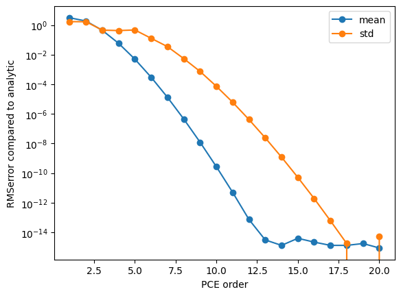
[11]:
# plot the convergence of the mean and standard deviation to that of the highest order

mean_analytic = exact['expectation']
std_analytic = np.sqrt(exact['variance'])

O = [R[r]['order'] for r in list(R.keys())]
plt.figure()
plt.semilogy([o for o in O],
             [np.abs(R[o]['results'].describe('Ishigami', 'mean') - mean_analytic) for o in O],
             'o-', label='mean')
plt.semilogy([o for o in O],
             [np.abs(R[o]['results'].describe('Ishigami', 'std') - std_analytic) for o in O],
             'o-', label='std')
plt.xlabel('PCE order')
plt.ylabel('RMSerror compared to analytic')
plt.legend(loc=0)
plt.savefig('Convergence_mean_std.png')
plt.savefig('Convergence_mean_std.pdf')
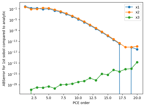
[12]:
# plot the convergence of the first sobol to that of the highest order

sobol_first_exact = {'x1': exact['S1'], 'x2': exact['S2'], 'x3': exact['S3']}

O = [R[r]['order'] for r in list(R.keys())]
plt.figure()
for v in list(R[O[0]]['results'].sobols_first('Ishigami').keys()):
    plt.semilogy([o for o in O],
                 [np.abs(R[o]['results'].sobols_first('Ishigami')[v] - sobol_first_exact[v]) for o in O],
                 'o-',
                 label=v)
plt.xlabel('PCE order')
plt.ylabel('ABSerror for 1st sobol compared to analytic')
plt.legend(loc=0)
plt.savefig('Convergence_sobol_first.png')
plt.savefig('Convergence_sobol_first.pdf')
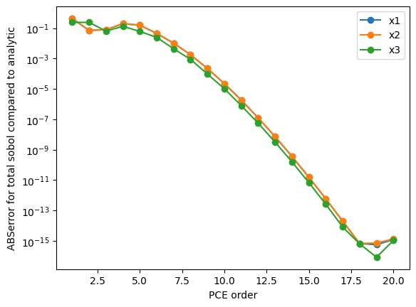
[13]:
# plot the convergence of the total sobol to that of the highest order

sobol_total_exact = {'x1': exact['ST1'], 'x2': exact['ST2'], 'x3': exact['ST3']}

O = [R[r]['order'] for r in list(R.keys())]
plt.figure()
for v in list(R[O[0]]['results'].sobols_total('Ishigami').keys()):
    plt.semilogy([o for o in O],
                 [np.abs(R[o]['results'].sobols_total('Ishigami')[v] - sobol_total_exact[v]) for o in O],
                 'o-',
                 label=v)
plt.xlabel('PCE order')
plt.ylabel('ABSerror for total sobol compared to analytic')
plt.legend(loc=0)
plt.savefig('Convergence_sobol_total.png')
plt.savefig('Convergence_sobol_total.pdf')
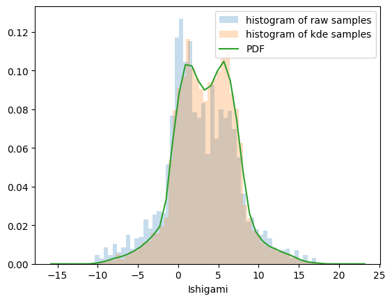
[14]:
# Plot the distribution function

results_df = R[O[-1]]['results_df']
results = R[O[-1]]['results']
Ishigami_dist = results.raw_data['output_distributions']['Ishigami']

plt.figure()
plt.hist(results_df.Ishigami[0], density=True, bins=50, label='histogram of raw samples', alpha=0.25)
if hasattr(Ishigami_dist, 'samples'):
    plt.hist(Ishigami_dist.samples[0], density=True, bins=50, label='histogram of kde samples', alpha=0.25)
t1 = Ishigami_dist[0]
plt.plot(np.linspace(t1.lower, t1.upper), t1.pdf(np.linspace(t1.lower,t1.upper)), label='PDF')
plt.legend(loc=0)
plt.xlabel('Ishigami')
plt.savefig('Ishigami_distribution_function.png')
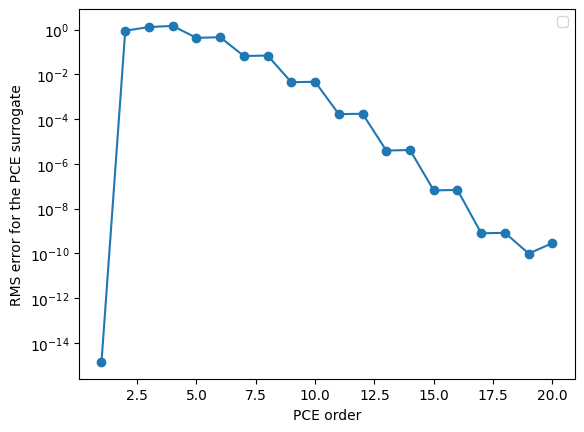
[15]:
# plot the RMS surrogate error at the PCE vary points
_o = []
_RMS = []
for r in R.values():
    results_df = r['results_df']
    results = r['results']
    Ishigami_surrogate = np.squeeze(np.array(results.surrogate()(results_df[results.inputs])['Ishigami']))
    Ishigami_samples = np.squeeze(np.array(results_df['Ishigami']))
    _RMS.append((np.sqrt((((Ishigami_surrogate - Ishigami_samples))**2).mean())))
    _o.append(r['order'])

plt.figure()
plt.semilogy(_o, _RMS, 'o-')
plt.xlabel('PCE order')
plt.ylabel('RMS error for the PCE surrogate')
plt.legend(loc=0)
plt.savefig('Convergence_surrogate.png')
plt.savefig('Convergence_surrogate.pdf')
/var/folders/6f/rn14629n60j16dc99dtk7bs4000ctx/T/ipykernel_71217/3184545625.py:16: UserWarning: No artists with labels found to put in legend.  Note that artists whose label start with an underscore are ignored when legend() is called with no argument.
  plt.legend(loc=0)
[16]:
# prepare the test data
test_campaign = uq.Campaign(name='Ishigami.')
test_campaign.add_app(name="Ishigami", params=define_params(),
                      actions=uq.actions.Actions(uq.actions.ExecutePython(run_ishigami_model)))
test_campaign.set_sampler(uq.sampling.quasirandom.LHCSampler(vary=define_vary(), count=100))
test_campaign.execute(nsamples=1000, sequential=True).collate(progress_bar=True)
test_df = test_campaign.get_collation_result()
100%|█████████████████████████████████████| 1000/1000 [00:00<00:00, 6585.05it/s]
[17]:
# calculate the PCE surrogates
test_points = test_df[test_campaign.get_active_sampler().vary.get_keys()]
test_results = np.squeeze(test_df['Ishigami'].values)
test_predictions = {}
for i in list(R.keys()):
    test_predictions[i] = np.squeeze(np.array(R[i]['results'].surrogate()(test_points)['Ishigami']))
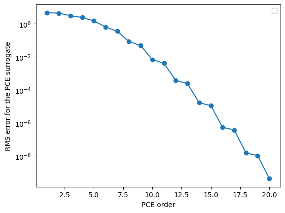
[18]:
# plot the convergence of the surrogate
_o = []
_RMS = []
for r in R.values():
    _RMS.append((np.sqrt((((test_predictions[r['order']] - test_results))**2).mean())))
    _o.append(r['order'])

plt.figure()
plt.semilogy(_o, _RMS, 'o-')
plt.xlabel('PCE order')
plt.ylabel('RMS error for the PCE surrogate')
plt.legend(loc=0)
plt.savefig('Convergence_PCE_surrogate.png')
plt.savefig('Convergence_PCE_surrogate.pdf')
/var/folders/6f/rn14629n60j16dc99dtk7bs4000ctx/T/ipykernel_71217/3799094119.py:12: UserWarning: No artists with labels found to put in legend.  Note that artists whose label start with an underscore are ignored when legend() is called with no argument.
  plt.legend(loc=0)
[ ]: