Run the fusion EasyVVUQ campaign using SC

Run an EasyVVUQ campaign to analyze the sensitivity of the temperature profile predicted by a simplified model of heat conduction in a tokamak plasma.

This is done with SC.

# import packages that we will use
%matplotlib inline
import os
import easyvvuq as uq
import chaospy as cp
import pickle
import time
import numpy as np
import pandas as pd
import matplotlib
if not os.getenv("DISPLAY"): matplotlib.use('Agg')
import matplotlib.pylab as plt
from IPython.display import display
%matplotlib inline

/Volumes/UserData/dpc/GIT/EasyVVUQ/env_3.12/lib/python3.12/site-packages/chaospy/__init__.py:9: UserWarning: pkg_resources is deprecated as an API. See https://setuptools.pypa.io/en/latest/pkg_resources.html. The pkg_resources package is slated for removal as early as 2025-11-30. Refrain from using this package or pin to Setuptools<81.
  import pkg_resources

# we need fipy -- install if not already available

try:
    import fipy
except ModuleNotFoundError:
    ! pip install future
    ! pip install fipy
    import fipy

# routine to write out (if needed) the fusion .template file

def write_template(params):
    str = ""
    first = True
    for k in params.keys():
        if first:
            str += '{"%s": "$%s"' % (k,k) ; first = False
        else:
            str += ', "%s": "$%s"' % (k,k)
    str += '}'
    print(str, file=open('fusion.template','w'))

# define parameters of the fusion model
def define_params():
    return {
        "Qe_tot":   {"type": "float",   "min": 1.0e6, "max": 50.0e6, "default": 2e6},
        "H0":       {"type": "float",   "min": 0.00,  "max": 1.0,    "default": 0},
        "Hw":       {"type": "float",   "min": 0.01,  "max": 100.0,  "default": 0.1},
        "Te_bc":    {"type": "float",   "min": 10.0,  "max": 1000.0, "default": 100},
        "chi":      {"type": "float",   "min": 0.01,  "max": 100.0,  "default": 1},
        "a0":       {"type": "float",   "min": 0.2,   "max": 10.0,   "default": 1},
        "R0":       {"type": "float",   "min": 0.5,   "max": 20.0,   "default": 3},
        "E0":       {"type": "float",   "min": 1.0,   "max": 10.0,   "default": 1.5},
        "b_pos":    {"type": "float",   "min": 0.95,  "max": 0.99,   "default": 0.98},
        "b_height": {"type": "float",   "min": 3e19,  "max": 10e19,  "default": 6e19},
        "b_sol":    {"type": "float",   "min": 2e18,  "max": 3e19,   "default": 2e19},
        "b_width":  {"type": "float",   "min": 0.005, "max": 0.025,  "default": 0.01},
        "b_slope":  {"type": "float",   "min": 0.0,   "max": 0.05,   "default": 0.01},
        "nr":       {"type": "integer", "min": 10,    "max": 1000,   "default": 100},
        "dt":       {"type": "float",   "min": 1e-3,  "max": 1e3,    "default": 100},
        "out_file": {"type": "string",  "default": "output.csv"}
    }

# define varying quantities
def define_vary():
    vary_all = {
        "Qe_tot":   cp.Uniform(1.8e6, 2.2e6),
        "H0":       cp.Uniform(0.0,   0.2),
        "Hw":       cp.Uniform(0.1,   0.5),
        "chi":      cp.Uniform(0.8,   1.2),
        "Te_bc":    cp.Uniform(80.0,  120.0),
        "a0":       cp.Uniform(0.9,   1.1),
        "R0":       cp.Uniform(2.7,   3.3),
        "E0":       cp.Uniform(1.4,   1.6),
        "b_pos":    cp.Uniform(0.95,  0.99),
        "b_height": cp.Uniform(5e19,  7e19),
        "b_sol":    cp.Uniform(1e19,  3e19),
        "b_width":  cp.Uniform(0.015, 0.025),
        "b_slope":  cp.Uniform(0.005, 0.020)
    }
    vary_2 =  {
        "Qe_tot":   cp.Uniform(1.8e6, 2.2e6),
        "Te_bc":    cp.Uniform(80.0,  120.0)
    }
    vary_5 =  {
        "Qe_tot":   cp.Uniform(1.8e6, 2.2e6),
        "H0":       cp.Uniform(0.0,   0.2),
        "Hw":       cp.Uniform(0.1,   0.5),
        "chi":      cp.Uniform(0.8,   1.2),
        "Te_bc":    cp.Uniform(80.0,  120.0)
    }
    vary_10 = {
        "Qe_tot":   cp.Uniform(1.8e6, 2.2e6),
        "H0":       cp.Uniform(0.0,   0.2),
        "Hw":       cp.Uniform(0.1,   0.5),
        "chi":      cp.Uniform(0.8,   1.2),
        "Te_bc":    cp.Uniform(80.0,  120.0),
        "b_pos":    cp.Uniform(0.95,  0.99),
        "b_height": cp.Uniform(5e19,  7e19),
        "b_sol":    cp.Uniform(1e19,  3e19),
        "b_width":  cp.Uniform(0.015, 0.025),
        "b_slope":  cp.Uniform(0.005, 0.020)
    }
    return vary_5

# define a model to run the fusion code directly from python, expecting a dictionary and returning a dictionary
def run_fusion_model(input):
    import json
    import fusion
    qois = ["te", "ne", "rho", "rho_norm"]
    del input['out_file']
    return {q: v for q,v in zip(qois, [t.tolist() for t in fusion.solve_Te(**input, plots=False, output=False)])}

# routine to run a SC campaign

def run_sc_case(sc_order=2, local=True, dask=True, batch_size=os.cpu_count(), use_files=True):
    """
    Inputs:
        sc_order: order of the sc expansion
        local: if using Dask, whether to use the local option (True)
        dask: whether to use dask (True)
        batch_size: for the non Dask option, number of cases to run in parallel (16)
    Outputs:
        results_df: Pandas dataFrame containing inputs to and output from the model
        results: Results of the sc analysis
        times: Information about the elapsed time for the various phases of the calculation
        sc_order: sc_order
        count: number of sc samples
    """

    if dask:
        if local:
            print('Running locally')
            import multiprocessing.popen_spawn_posix
            from dask.distributed import Client, LocalCluster
            cluster = LocalCluster(threads_per_worker=1)
            client = Client(cluster) # processes=True, threads_per_worker=1)
        else:
            print('Running using SLURM')
            from dask.distributed import Client
            from dask_jobqueue import SLURMCluster
            cluster = SLURMCluster(
                job_extra=['--qos=p.tok.openmp.2h', '--mail-type=end', '--mail-user=dpc@rzg.mpg.de', '-t 2:00:00'],
                queue='p.tok.openmp',
                cores=8,
                memory='8 GB',
                processes=8)
            cluster.scale(32)
            print(cluster)
            print(cluster.job_script())
            client = Client(cluster)
        print(client)

    else:
        import concurrent.futures
#        client = concurrent.futures.ProcessPoolExecutor(max_workers=batch_size)
        client = concurrent.futures.ThreadPoolExecutor(max_workers=batch_size)
#        client = None

    times = np.zeros(7)

    time_start = time.time()
    time_start_whole = time_start
    # Set up a fresh campaign called "fusion_sc."
    my_campaign = uq.Campaign(name='fusion_sc.')

    # Define parameter space
    params = define_params()

    # Create an encoder and decoder for sc test app
    if use_files:
        encoder = uq.encoders.GenericEncoder(template_fname='fusion.template',
                                             delimiter='$',
                                             target_filename='fusion_in.json')


        decoder = uq.decoders.SimpleCSV(target_filename="output.csv",
                                        output_columns=["te", "ne", "rho", "rho_norm"])

        execute = uq.actions.ExecuteLocal('python3 %s/fusion_model.py fusion_in.json' % (os.getcwd()))

        actions = uq.actions.Actions(uq.actions.CreateRunDirectory('/tmp'),
                                     uq.actions.Encode(encoder), execute, uq.actions.Decode(decoder))
    else:
        actions = uq.actions.Actions(uq.actions.ExecutePython(run_fusion_model))


    # Add the app (automatically set as current app)
    my_campaign.add_app(name="fusion", params=params, actions=actions)

    time_end = time.time()
    times[1] = time_end-time_start
    print('Time for phase 1 = %.3f' % (times[1]))

    time_start = time.time()
    # Associate a sampler with the campaign
    my_campaign.set_sampler(uq.sampling.SCSampler(vary=define_vary(), polynomial_order=sc_order))
    my_campaign.draw_samples()
    print('Number of samples = %s' % my_campaign.get_active_sampler().count)

    time_end = time.time()
    times[2] = time_end-time_start
    print('Time for phase 2 = %.3f' % (times[2]))

    time_start = time.time()
    # Perform the actions
    my_campaign.execute(pool=client).collate(progress_bar=True)

    if dask:
        client.close()
        client.shutdown()

    time_end = time.time()
    times[3] = time_end-time_start
    print('Time for phase 3 = %.3f' % (times[3]))

    time_start = time.time()
    # Collate the results
    results_df = my_campaign.get_collation_result()

    time_end = time.time()
    times[4] = time_end-time_start
    print('Time for phase 4 = %.3f' % (times[4]))

    time_start = time.time()
    # Post-processing analysis
    results = my_campaign.analyse(qoi_cols=["te", "ne", "rho", "rho_norm"])

    time_end = time.time()
    times[5] = time_end-time_start
    print('Time for phase 5 = %.3f' % (times[5]))

    time_start = time.time()
    # Save the results
    pickle.dump(results, open('fusion_results.pickle','bw'))
    time_end = time.time()
    times[6] = time_end-time_start
    print('Time for phase 6 = %.3f' % (times[6]))

    times[0] = time_end - time_start_whole

    return results_df, results, times, sc_order, my_campaign.get_active_sampler().count

# routines for plotting the results

def plot_Te(results, title=None):
    # plot the calculated Te: mean, with std deviation, 1, 10, 90 and 99%
    plt.figure()
    rho = results.describe('rho', 'mean')
    plt.plot(rho, results.describe('te', 'mean'), 'b-', label='Mean')
    plt.plot(rho, results.describe('te', 'mean')-results.describe('te', 'std'), 'b--', label='+1 std deviation')
    plt.plot(rho, results.describe('te', 'mean')+results.describe('te', 'std'), 'b--')
    plt.fill_between(rho, results.describe('te', 'mean')-results.describe('te', 'std'), results.describe('te', 'mean')+results.describe('te', 'std'), color='b', alpha=0.2)
    try:
        plt.plot(rho, results.describe('te', '10%'), 'b:', label='10 and 90 percentiles')
        plt.plot(rho, results.describe('te', '90%'), 'b:')
        plt.fill_between(rho, results.describe('te', '10%'), results.describe('te', '90%'), color='b', alpha=0.1)
        plt.fill_between(rho, results.describe('te', '1%'), results.describe('te', '99%'), color='b', alpha=0.05)
    except:
        print('Problem with some of the percentiles')
    plt.legend(loc=0)
    plt.xlabel('rho [$m$]')
    plt.ylabel('Te [$eV$]')
    if not title is None: plt.title(title)
    plt.savefig('Te.png')
    plt.savefig('Te.pdf')

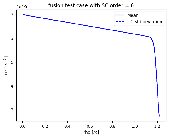
def plot_ne(results, title=None):
    # plot the calculated ne: mean, with std deviation, 1, 10, 90 and 99%
    plt.figure()
    rho = results.describe('rho', 'mean')
    plt.plot(rho, results.describe('ne', 'mean'), 'b-', label='Mean')
    plt.plot(rho, results.describe('ne', 'mean')-results.describe('ne', 'std'), 'b--', label='+1 std deviation')
    plt.plot(rho, results.describe('ne', 'mean')+results.describe('ne', 'std'), 'b--')
    plt.fill_between(rho, results.describe('ne', 'mean')-results.describe('ne', 'std'), results.describe('ne', 'mean')+results.describe('ne', 'std'), color='b', alpha=0.2)
    try:
        plt.plot(rho, results.describe('ne', '10%'), 'b:', label='10 and 90 percentiles')
        plt.plot(rho, results.describe('ne', '90%'), 'b:')
        plt.fill_between(rho, results.describe('ne', '10%'), results.describe('ne', '90%'), color='b', alpha=0.1)
        plt.fill_between(rho, results.describe('ne', '1%'), results.describe('ne', '99%'), color='b', alpha=0.05)
    except:
        print('Problem with some of the percentiles')
    plt.legend(loc=0)
    plt.xlabel('rho [$m$]')
    plt.ylabel('ne [$m^{-3}$]')
    if not title is None: plt.title(title)
    plt.savefig('ne.png')
    plt.savefig('ne.pdf')

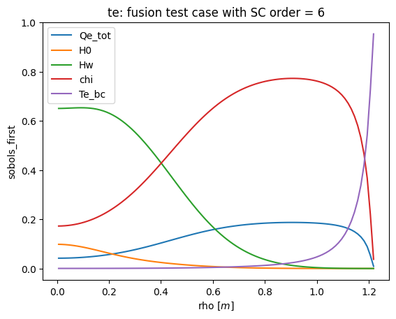
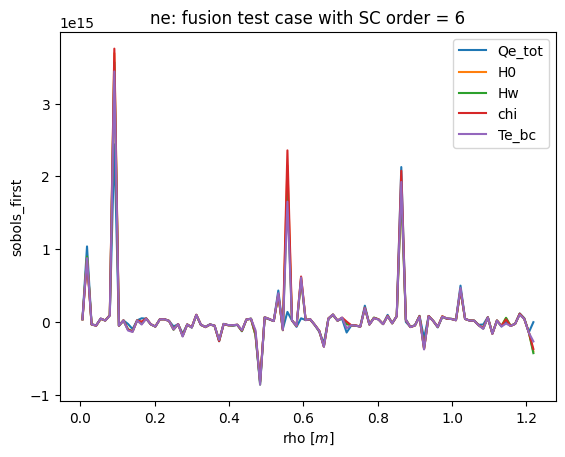
def plot_sobols_first(results, title=None, field='te'):
    # plot the first Sobol results
    plt.figure()
    rho = results.describe('rho', 'mean')
    for k in results.sobols_first()[field].keys(): plt.plot(rho, results.sobols_first()[field][k], label=k)
    plt.legend(loc=0)
    plt.xlabel('rho [$m$]')
    plt.ylabel('sobols_first')
    if not title is None: plt.title(field + ': ' + title)
    plt.savefig('sobols_first_%s.png' % (field))
    plt.savefig('sobols_first_%s.pdf' % (field))

def plot_sobols_second(results, title=None, field='te'):
    # plot the second Sobol results
    plt.figure()
    rho = results.describe('rho', 'mean')
    for k1 in results.sobols_second()[field].keys():
        for k2 in results.sobols_second()[field][k1].keys():
            plt.plot(rho, results.sobols_second()[field][k1][k2], label=k1+'/'+k2)
    plt.legend(loc=0, ncol=2)
    plt.xlabel('rho [$m$]')
    plt.ylabel('sobols_second')
    if not title is None: plt.title(field + ': ' + title)
    plt.savefig('sobols_second_%s.png' % (field))
    plt.savefig('sobols_second_%s.pdf' % (field))

def plot_sobols_total(results, title=None, field='te'):
    # plot the total Sobol results
    plt.figure()
    rho = results.describe('rho', 'mean')
    for k in results.sobols_total()[field].keys(): plt.plot(rho, results.sobols_total()[field][k], label=k)
    plt.legend(loc=0)
    plt.xlabel('rho [$m$]')
    plt.ylabel('sobols_total')
    if not title is None: plt.title(field + ': ' + title)
    plt.savefig('sobols_total_%s.png' % (field))
    plt.savefig('sobols_total_%s.pdf' % (field))

def plot_distribution(results, results_df, title=None):
    te_dist = results.raw_data['output_distributions']['te']
    rho_norm = results.describe('rho_norm', 'mean')
    for i in [np.maximum(0, int(i-1))
              for i in np.linspace(0,1,5) * rho_norm.shape]:
        plt.figure()
        pdf_raw_samples = cp.GaussianKDE(results_df.te[i])
        pdf_kde_samples = cp.GaussianKDE(te_dist.samples[i])
        plt.hist(results_df.te[i], density=True, bins=50, label='histogram of raw samples', alpha=0.25)
        if hasattr(te_dist, 'samples'):
            plt.hist(te_dist.samples[i], density=True, bins=50, label='histogram of kde samples', alpha=0.25)

        plt.plot(np.linspace(pdf_raw_samples.lower, pdf_raw_samples.upper), pdf_raw_samples.pdf(np.linspace(pdf_raw_samples.lower, pdf_raw_samples.upper)), label='PDF (raw samples)')
        plt.plot(np.linspace(pdf_kde_samples.lower, pdf_kde_samples.upper), pdf_kde_samples.pdf(np.linspace(pdf_kde_samples.lower, pdf_kde_samples.upper)), label='PDF (kde samples)')

        plt.legend(loc=0)
        plt.xlabel('Te [$eV$]')
        if title is None:
            plt.title('Distributions for rho_norm = %0.4f' % (rho_norm[i]))
        else:
            plt.title('%s\nDistributions for rho_norm = %0.4f' % (title, rho_norm[i]))
        plt.savefig('distribution_function_rho_norm=%0.4f.png' % (rho_norm[i]))
        plt.savefig('distribution_function_rho_norm=%0.4f.pdf' % (rho_norm[i]))

# Calculate the stochastic collocation expansion for a range of orders

if __name__ == '__main__':
    local = False        # if True, use local cores; if False, use SLURM
    dask = False         # if True, use DASK; if False, use a fall-back non-DASK option

    R = {}
    for sc_order in range(1, 7):
        R[sc_order] = {}
        (R[sc_order]['results_df'],
         R[sc_order]['results'],
         R[sc_order]['times'],
         R[sc_order]['order'],
         R[sc_order]['number_of_samples']) = run_sc_case(sc_order=sc_order,
                                                           local=local, dask=dask,
                                                           batch_size=7, use_files=False)

/Volumes/UserData/dpc/GIT/EasyVVUQ/env_3.12/lib/python3.12/site-packages/cerberus/validator.py:618: UserWarning: These types are defined both with a method and in the'types_mapping' property of this validator: {'integer'}
  warn(
/Volumes/UserData/dpc/GIT/EasyVVUQ/env_3.12/lib/python3.12/site-packages/cerberus/validator.py:618: UserWarning: These types are defined both with a method and in the'types_mapping' property of this validator: {'integer'}
  warn(

Time for phase 1 = 0.017
Number of samples = 32
Time for phase 2 = 0.035

100%|██████████████████████████████████████████████████████████████████████████████████████████████████████████████████████████████████████████████████████████████████████████████████████████████████████████████████████████████████████████████████████████████████████████████████████████| 32/32 [00:00<00:00, 74.02it/s]

Time for phase 3 = 0.448
Time for phase 4 = 0.006
Time for phase 5 = 0.030
Time for phase 6 = 0.001
Time for phase 1 = 0.005
Number of samples = 243
Time for phase 2 = 0.115

100%|████████████████████████████████████████████████████████████████████████████████████████████████████████████████████████████████████████████████████████████████████████████████████████████████████████████████████████████████████████████████████████████████████████████████████████| 243/243 [00:02<00:00, 88.70it/s]

Time for phase 3 = 3.087
Time for phase 4 = 0.024
Time for phase 5 = 0.214
Time for phase 6 = 0.002
Time for phase 1 = 0.004
Number of samples = 1024
Time for phase 2 = 0.381

100%|██████████████████████████████████████████████████████████████████████████████████████████████████████████████████████████████████████████████████████████████████████████████████████████████████████████████████████████████████████████████████████████████████████████████████████| 1024/1024 [00:12<00:00, 80.66it/s]

Time for phase 3 = 13.070
Time for phase 4 = 0.097
Time for phase 5 = 1.204
Time for phase 6 = 0.010
Time for phase 1 = 0.006
Number of samples = 3125
Time for phase 2 = 1.143

100%|██████████████████████████████████████████████████████████████████████████████████████████████████████████████████████████████████████████████████████████████████████████████████████████████████████████████████████████████████████████████████████████████████████████████████████| 3125/3125 [00:39<00:00, 78.79it/s]

Time for phase 3 = 40.277
Time for phase 4 = 0.287
Time for phase 5 = 6.339
Time for phase 6 = 0.023
Time for phase 1 = 0.005
Number of samples = 7776
Time for phase 2 = 2.637

100%|██████████████████████████████████████████████████████████████████████████████████████████████████████████████████████████████████████████████████████████████████████████████████████████████████████████████████████████████████████████████████████████████████████████████████████| 7776/7776 [01:39<00:00, 77.86it/s]

Time for phase 3 = 100.147
Time for phase 4 = 0.747
Time for phase 5 = 28.585
Time for phase 6 = 0.057
Time for phase 1 = 0.004
Number of samples = 16807
Time for phase 2 = 5.628

100%|████████████████████████████████████████████████████████████████████████████████████████████████████████████████████████████████████████████████████████████████████████████████████████████████████████████████████████████████████████████████████████████████████████████████████| 16807/16807 [03:33<00:00, 78.86it/s]

Time for phase 3 = 213.790
Time for phase 4 = 1.743
Time for phase 5 = 121.002
Time for phase 6 = 0.131

# save the results

if __name__ == '__main__':

    pickle.dump(R, open('collected_results.pickle','bw'))

# produce a table of the time taken for various phases
# the phases are:
#   1: creation of campaign
#   2: creation of samples
#   3: running the cases
#   4: calculation of statistics including Sobols
#   5: returning of analysed results
#   6: saving campaign and pickled results

if __name__ == '__main__':

    Timings = pd.DataFrame(np.array([R[r]['times'] for r in list(R.keys())]),
                 columns=['Total', 'Phase 1', 'Phase 2', 'Phase 3', 'Phase 4', 'Phase 5', 'Phase 6'],
                 index=[R[r]['order'] for r in list(R.keys())])
    Timings.to_csv(open('Timings.csv', 'w'))
    display(Timings)

	Total	Phase 1	Phase 2	Phase 3	Phase 4	Phase 5	Phase 6
1	0.536658	0.017182	0.034876	0.448066	0.006149	0.029729	0.000557
2	3.446937	0.004853	0.114904	3.087407	0.024183	0.213731	0.001767
3	14.766615	0.004219	0.381222	13.070184	0.096659	1.204292	0.009901
4	48.073970	0.005606	1.143053	40.276773	0.286804	6.338882	0.022661
5	132.179250	0.004542	2.637365	100.147288	0.747055	28.585327	0.057435
6	342.298249	0.004455	5.628100	213.790076	1.743332	121.001515	0.130513

# plot the convergence of the mean and standard deviation to that of the highest order

if __name__ == '__main__':
    last = -1
    O = [R[r]['order'] for r in list(R.keys())]
    if len(O[0:last]) > 0:
        plt.figure()
        plt.semilogy([o for o in O[0:last]],
                     [np.sqrt(np.mean((R[o]['results'].describe('te', 'mean') -
                                       R[O[last]]['results'].describe('te', 'mean'))**2)) for o in O[0:last]],
                     'o-', label='mean')
        plt.semilogy([o for o in O[0:last]],
                     [np.sqrt(np.mean((R[o]['results'].describe('te', 'std') -
                                       R[O[last]]['results'].describe('te', 'std'))**2)) for o in O[0:last]],
                     'o-', label='std')
        plt.xlabel('SC order')
        plt.ylabel('RMSerror compared to order=%s' % (O[last]))
        plt.legend(loc=0)
        plt.savefig('Convergence_mean_std.png')
        plt.savefig('Convergence_mean_std.pdf')

# plot the convergence of the first sobol to that of the highest order

if __name__ == '__main__':
    last = -1
    O = [R[r]['order'] for r in list(R.keys())]
    if len(O[0:last]) > 0:
        plt.figure()
        O = [R[r]['order'] for r in list(R.keys())]
        for v in list(R[O[last]]['results'].sobols_first('te').keys()):
            plt.semilogy([o for o in O[0:last]],
                         [np.sqrt(np.mean((R[o]['results'].sobols_first('te')[v] -
                                           R[O[last]]['results'].sobols_first('te')[v])**2)) for o in O[0:last]],
                         'o-',
                         label=v)
        plt.xlabel('SC order')
        plt.ylabel('RMSerror for 1st sobol compared to order=%s' % (O[last]))
        plt.legend(loc=0)
        plt.savefig('Convergence_sobol_first.png')
        plt.savefig('Convergence_sobol_first.pdf')

# plot a standard set of graphs for the highest order case

if __name__ == '__main__':
    last = -1
    title = 'fusion test case with SC order = %i' % list(R.values())[last]['order']
    plot_Te(list(R.values())[last]['results'], title=title,)
    plot_ne(list(R.values())[last]['results'], title=title)
    plot_sobols_first(list(R.values())[last]['results'], title=title)
    try:
        plot_sobols_second(list(R.values())[last]['results'], title=title)
    except:
        print('Problem with sobols_second')
    try:
        plot_sobols_total(list(R.values())[last]['results'], title=title)
    except:
        print('Problem with sobols_total')
    try:
        plot_distribution(list(R.values())[last]['results'], list(R.values())[last]['results_df'], title=title)
    except:
        print('Problem with distribution')
    plot_sobols_first(list(R.values())[last]['results'], title=title, field='ne')
    try:
        plot_sobols_second(list(R.values())[last]['results'], title=title, field='ne')
    except:
        print('Problem with sobols_second')
    try:
        plot_sobols_total(list(R.values())[last]['results'], title=title, field='ne')
    except:
        print('Problem with sobols_total')

Problem with some of the percentiles
Problem with some of the percentiles
Problem with sobols_second
Problem with sobols_total
Problem with distribution
Problem with sobols_second
Problem with sobols_total

<Figure size 640x480 with 0 Axes>

<Figure size 640x480 with 0 Axes>

<Figure size 640x480 with 0 Axes>

<Figure size 640x480 with 0 Axes>

# prepare the test data

if __name__ == '__main__':

    test_campaign = uq.Campaign(name='fusion_pce.')

    # Add the app (automatically set as current app)
    test_campaign.add_app(name="fusion", params=define_params(),
                          actions=uq.actions.Actions(uq.actions.ExecutePython(run_fusion_model)))

    # Associate a sampler with the campaign
    test_campaign.set_sampler(uq.sampling.quasirandom.LHCSampler(vary=define_vary(), count=100))

    # Perform the actions
    test_campaign.execute(nsamples=1000).collate(progress_bar=True)

    # Collate the results
    test_df = test_campaign.get_collation_result()

100%|██████████████████████████████████████████████████████████████████████████████████████████████████████████████████████████████████████████████████████████████████████████████████████████████████████████████████████████████████████████████████████████████████████████████████████| 1000/1000 [00:12<00:00, 78.51it/s]

# calculate the SC surrogates
if __name__ == '__main__':

    test_points = test_df[test_campaign.get_active_sampler().vary.get_keys()]
    test_results = test_df['te'].values
    test_predictions = {}
    for i in list(R.keys()):
        test_predictions[i] = np.squeeze(np.array(R[i]['results'].surrogate()(test_points)['te']))

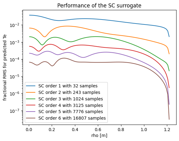
# plot the performance of the SC surrogates
if __name__ == '__main__':

    for i in list(R.keys()):
        plt.semilogy(R[i]['results'].describe('rho', 'mean'),
                 np.sqrt(((test_predictions[i] - test_results)**2).mean(axis=0)) / test_results.mean(axis=0),
                 label='SC order %s with %s samples' % (R[i]['order'], R[i]['number_of_samples']))
    plt.xlabel('rho [m]') ; plt.ylabel('fractional RMS for predicted Te') ; plt.legend(loc=0)
    plt.title('Performance of the SC surrogate')
    plt.savefig('SC_surrogate.png')
    plt.savefig('SC_surrogate.pdf')

# plot the convergence of the surrogate based on 1000 random points
if __name__ == '__main__':
    _o = []
    _RMS = []
    for r in R.values():
        _RMS.append((np.sqrt((((test_predictions[r['order']] - test_results) / test_results)**2).mean())))
        _o.append(r['order'])

    plt.figure()
    plt.semilogy(_o, _RMS, 'o-')
    plt.xlabel('SC order')
    plt.ylabel('fractional RMS error for the SC surrogate')
    plt.legend(loc=0)
    plt.savefig('Convergence_SC_surrogate.png')
    plt.savefig('Convergence_SC_surrogate.pdf')

/var/folders/_0/dx4n8sh94h107t1d3g7wjwbm0000gn/T/ipykernel_4774/2909014312.py:13: UserWarning: No artists with labels found to put in legend.  Note that artists whose label start with an underscore are ignored when legend() is called with no argument.
  plt.legend(loc=0)