Sensityivity analysis for the Ishigama function with noise using PCE

Run an EasyVVUQ campaign to analyze the sensitivity for the Ishigami function with noise

This is done with PCE providing a normal distributed noise value

[1]:

# Run an EasyVVUQ campaign to analyze the sensitivity for the Ishigami function with noise
# This is done with PCE providing a normal distributed noise value.
%matplotlib inline
import os
import easyvvuq as uq
import chaospy as cp
import pickle
import numpy as np
import matplotlib.pylab as plt
import time
import pandas as pd

[2]:

# Define the Ishigami function
def ishigamiSA(a,b):
    '''Exact sensitivity indices of the Ishigami function for given a and b.
    From https://openturns.github.io/openturns/master/examples/meta_modeling/chaos_ishigami.html
    '''
    var = 1.0/2 + a**2/8 + b*np.pi**4/5 + b**2*np.pi**8/18
    S1 = (1.0/2 + b*np.pi**4/5+b**2*np.pi**8/50)/var
    S2 = (a**2/8)/var
    S3 = 0
    S13 = b**2*np.pi**8/2*(1.0/9-1.0/25)/var
    exact = {
            'expectation' : a/2,
            'variance' : var,
            'S1' : (1.0/2 + b*np.pi**4/5+b**2*np.pi**8.0/50)/var,
            'S2' : (a**2/8)/var,
            'S3' : 0,
            'S12' : 0,
            'S23' : 0,
            'S13' : S13,
            'S123' : 0,
            'ST1' : S1 + S13,
            'ST2' : S2,
            'ST3' : S3 + S13
            }
    return exact

Ishigami_a = 7.0
Ishigami_b = 0.1
exact = ishigamiSA(Ishigami_a, Ishigami_b)

[3]:

# define a model to run the Ishigami code directly from python, expecting a dictionary and returning a dictionary
def run_ishigami_model(input):
    import Ishigami
    qois = ["Ishigami"]
    del input['out_file']
    N = input['N']
    del input['N']
    return {qois[0]: Ishigami.evaluate(**input)+N}

[4]:

# Define parameter space
def define_params():
    return {
        "x1":       {"type": "float",   "min": -np.pi,     "max": np.pi,      "default": 0.0},
        "x2":       {"type": "float",   "min": -np.pi,     "max": np.pi,      "default": 0.0},
        "x3":       {"type": "float",   "min": -np.pi,     "max": np.pi,      "default": 0.0},
        "a":        {"type": "float",   "min": Ishigami_a, "max": Ishigami_a, "default": Ishigami_a},
        "b":        {"type": "float",   "min": Ishigami_b, "max": Ishigami_b, "default": Ishigami_b},
        "N":        {"type": "float",   "min": -100.0,     "max": 100.0,      "default": 0.0},
        "out_file": {"type": "string",  "default": "output.csv"}
    }

[5]:

# Define varying space
def define_vary():
    return {
        "x1":   cp.Uniform(-np.pi, np.pi),
        "x2":   cp.Uniform(-np.pi, np.pi),
        "x3":   cp.Uniform(-np.pi, np.pi),
        "N":    cp.Normal(0, 10.0)
    }

[6]:

# Set up and run a campaign
def run_campaign(pce_order=2, use_files=False):

    times = np.zeros(7)

    time_start = time.time()
    time_start_whole = time_start

    # Set up a fresh campaign called "Ishigami_pce."
    my_campaign = uq.Campaign(name='Ishigami_pce.')

    # Create an encoder and decoder for PCE test app
    if use_files:
        encoder = uq.encoders.GenericEncoder(template_fname='Ishigami.template',
                                             delimiter='$',
                                             target_filename='Ishigami_in.json')

        decoder = uq.decoders.SimpleCSV(target_filename="output.csv",
                                        output_columns=["Ishigami"])

        execute = uq.actions.ExecuteLocal('python3 %s/Ishigami.py Ishigami_in.json' % (os.getcwd()))

        actions = uq.actions.Actions(uq.actions.CreateRunDirectory('/tmp'),
                          uq.actions.Encode(encoder), execute, uq.actions.Decode(decoder))
    else:
        actions = uq.actions.Actions(uq.actions.ExecutePython(run_ishigami_model))

    # Add the app (automatically set as current app)
    my_campaign.add_app(name="Ishigami", params=define_params(), actions=actions)

    # Create the sampler
    time_end = time.time()
    times[1] = time_end-time_start
    print('Time for phase 1 = %.3f' % (times[1]))

    time_start = time.time()
    # Associate a sampler with the campaign
    Sampler_PCE = uq.sampling.PCESampler(vary=define_vary(), polynomial_order=pce_order)
    my_campaign.set_sampler(Sampler_PCE)

    # Will draw all (of the finite set of samples)
    my_campaign.draw_samples()
    print('PCE order = %s' % pce_order)
    print('Number of samples = %s' % my_campaign.get_active_sampler().count)

    time_end = time.time()
    times[2] = time_end-time_start
    print('Time for phase 2 = %.3f' % (times[2]))

    time_start = time.time()
    # Run the cases
    my_campaign.execute(sequential=True).collate(progress_bar=True)

    time_end = time.time()
    times[3] = time_end-time_start
    print('Time for phase 3 = %.3f' % (times[3]))

    time_start = time.time()
    # Get the results
    results_df = my_campaign.get_collation_result()

    time_end = time.time()
    times[4] = time_end-time_start
    print('Time for phase 4 = %.3f' % (times[4]))

    time_start = time.time()
    # Post-processing analysis
    results = my_campaign.analyse(qoi_cols=["Ishigami"])

    time_end = time.time()
    times[5] = time_end-time_start
    print('Time for phase 5 = %.3f' % (times[5]))

    time_start = time.time()
    # Save the results
    pickle.dump(results, open('Ishigami_results.pickle','bw'))
    time_end = time.time()
    times[6] = time_end-time_start
    print('Time for phase 6 = %.3f' % (times[6]))

    times[0] = time_end - time_start_whole

    return results_df, results, times, pce_order, my_campaign.get_active_sampler().count

[7]:

# Calculate the polynomial chaos expansion for a range of orders

R = {}
for pce_order in range(1, 11):
    R[pce_order] = {}
    (R[pce_order]['results_df'],
     R[pce_order]['results'],
     R[pce_order]['times'],
     R[pce_order]['order'],
     R[pce_order]['number_of_samples']) = run_campaign(pce_order=pce_order, use_files=False)

Time for phase 1 = 0.034
PCE order = 1
Number of samples = 16
Time for phase 2 = 0.056

100%|█████████████████████████████████████████| 16/16 [00:00<00:00, 3128.04it/s]

Time for phase 3 = 0.030
Time for phase 4 = 0.004
Time for phase 5 = 0.041
Time for phase 6 = 0.002
Time for phase 1 = 0.007


Traceback (most recent call last):
  File "/Volumes/UserData/dpc/GIT/EasyVVUQ/env_3.12/lib/python3.12/site-packages/easyvvuq/analysis/pce_analysis.py", line 495, in analyse
    dY_hat = build_surrogate_der(fit, verbose=False)
             ^^^^^^^^^^^^^^^^^^^^^^^^^^^^^^^^^^^^^^^
  File "/Volumes/UserData/dpc/GIT/EasyVVUQ/env_3.12/lib/python3.12/site-packages/easyvvuq/analysis/pce_analysis.py", line 335, in build_surrogate_der
    assert(n1 == n2)
           ^^^^^^^^
AssertionError

PCE order = 2
Number of samples = 81
Time for phase 2 = 0.088

100%|█████████████████████████████████████████| 81/81 [00:00<00:00, 6073.81it/s]

Time for phase 3 = 0.019
Time for phase 4 = 0.002
Time for phase 5 = 0.133
Time for phase 6 = 0.001
Time for phase 1 = 0.007
PCE order = 3
Number of samples = 256
Time for phase 2 = 0.167

100%|███████████████████████████████████████| 256/256 [00:00<00:00, 6319.55it/s]

Time for phase 3 = 0.049
Time for phase 4 = 0.004

Time for phase 5 = 0.265
Time for phase 6 = 0.001
Time for phase 1 = 0.006
PCE order = 4
Number of samples = 625
Time for phase 2 = 0.370

100%|███████████████████████████████████████| 625/625 [00:00<00:00, 6280.84it/s]

Time for phase 3 = 0.115
Time for phase 4 = 0.008

Time for phase 5 = 0.642
Time for phase 6 = 0.011
Time for phase 1 = 0.007
PCE order = 5
Number of samples = 1296
Time for phase 2 = 0.520

100%|█████████████████████████████████████| 1296/1296 [00:00<00:00, 6776.62it/s]

Time for phase 3 = 0.220
Time for phase 4 = 0.016
Time for phase 5 = 1.636
Time for phase 6 = 0.001
Time for phase 1 = 0.006
PCE order = 6
Number of samples = 2401
Time for phase 2 = 0.989

100%|█████████████████████████████████████| 2401/2401 [00:00<00:00, 6610.41it/s]

Time for phase 3 = 0.419
Time for phase 4 = 0.026
Time for phase 5 = 5.114
Time for phase 6 = 0.002
Time for phase 1 = 0.018
PCE order = 7
Number of samples = 4096
Time for phase 2 = 1.599

100%|█████████████████████████████████████| 4096/4096 [00:00<00:00, 6753.46it/s]

Time for phase 3 = 0.753
Time for phase 4 = 0.040
Time for phase 5 = 15.794
Time for phase 6 = 0.004
Time for phase 1 = 0.014
PCE order = 8
Number of samples = 6561
Time for phase 2 = 3.132

100%|█████████████████████████████████████| 6561/6561 [00:01<00:00, 5595.64it/s]

Time for phase 3 = 1.328
Time for phase 4 = 0.134
Time for phase 5 = 34.943
Time for phase 6 = 0.006
Time for phase 1 = 0.022
PCE order = 9
Number of samples = 10000
Time for phase 2 = 3.888

100%|███████████████████████████████████| 10000/10000 [00:01<00:00, 5809.02it/s]

Time for phase 3 = 1.941
Time for phase 4 = 0.200
Time for phase 5 = 79.951
Time for phase 6 = 0.009
Time for phase 1 = 0.015
PCE order = 10
Number of samples = 14641
Time for phase 2 = 5.835

100%|███████████████████████████████████| 14641/14641 [00:02<00:00, 5799.49it/s]

Time for phase 3 = 2.988
Time for phase 4 = 0.259
Time for phase 5 = 182.045
Time for phase 6 = 0.016

[8]:

# save the results

pickle.dump(R, open('collected_results.pickle','bw'))

[9]:

# produce a table of the time taken for various phases
# the phases are:
#   1: creation of campaign
#   2: creation of samples
#   3: running the cases
#   4: calculation of statistics including Sobols
#   5: returning of analysed results
#   6: saving campaign and pickled results

Timings = pd.DataFrame(np.array([R[r]['times'] for r in list(R.keys())]),
             columns=['Total', 'Phase 1', 'Phase 2', 'Phase 3', 'Phase 4', 'Phase 5', 'Phase 6'],
             index=[R[r]['order'] for r in list(R.keys())])
Timings.to_csv(open('Timings.csv', 'w'))
display(Timings)

	Total	Phase 1	Phase 2	Phase 3	Phase 4	Phase 5	Phase 6
1	0.166434	0.034119	0.056325	0.029776	0.003714	0.040676	0.001628
2	0.250982	0.007045	0.088102	0.019497	0.002389	0.133038	0.000772
3	0.494265	0.007188	0.167473	0.049170	0.004417	0.264831	0.001052
4	1.152005	0.006146	0.369653	0.115196	0.008033	0.642317	0.010516
5	2.399874	0.006595	0.520325	0.220133	0.015788	1.635806	0.001044
6	6.555950	0.006280	0.988502	0.419108	0.025505	5.114128	0.002055
7	18.209050	0.017612	1.598959	0.753175	0.040242	15.793751	0.004482
8	39.557551	0.014352	3.131594	1.327839	0.134381	34.942869	0.005903
9	86.011995	0.022007	3.888345	1.941350	0.199872	79.950801	0.009002
10	191.162857	0.014980	5.835231	2.987610	0.258682	182.044722	0.016074

[10]:

R[10]['results'].plot_sobols_treemap('Ishigami')

/Volumes/UserData/dpc/GIT/EasyVVUQ/env_3.12/lib/python3.12/site-packages/easyvvuq/analysis/results.py:467: UserWarning: FigureCanvasAgg is non-interactive, and thus cannot be shown
  fig.show()

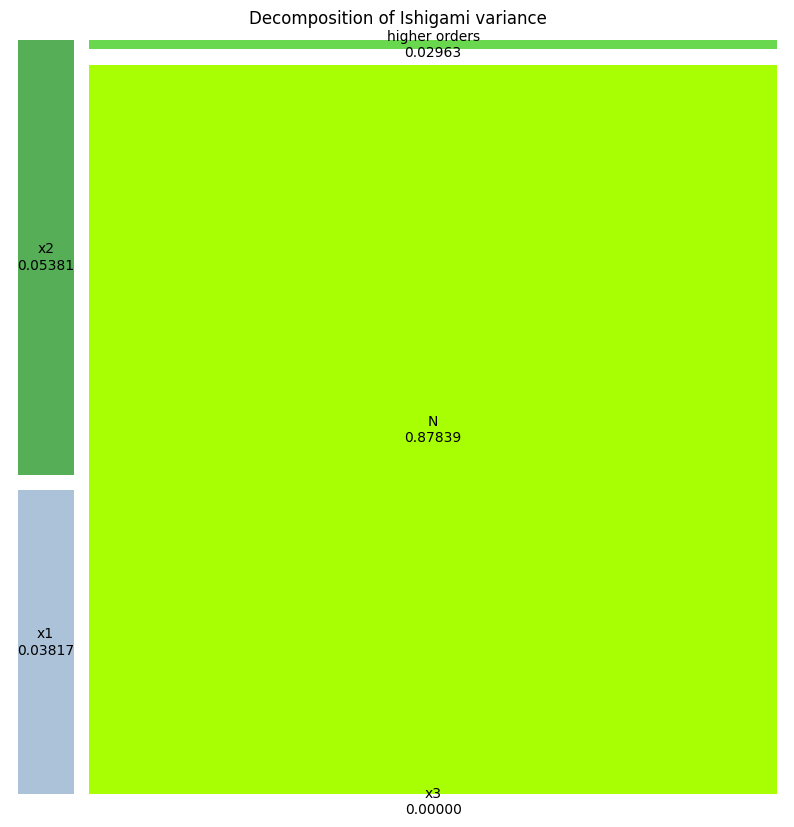
../_images/tutorials_easyvvuq_Ishigami_with_noise_tutorial_10_1.png

[11]:

R[10]['results'].sobols_first(), R[10]['results'].sobols_total()

[11]:

({'Ishigami': {'x1': array([0.03817368]),
   'x2': array([0.05380603]),
   'x3': array([1.28773622e-29]),
   'N': array([0.87838626])}},
 {'Ishigami': {'x1': array([0.06780771]),
   'x2': array([0.05380603]),
   'x3': array([0.02963403]),
   'N': array([0.87838626])}})

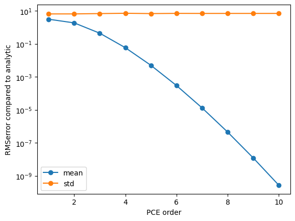
[12]:

# plot the convergence of the mean and standard deviation to the analytic result

mean_analytic = exact['expectation']
std_analytic = np.sqrt(exact['variance'])

O = [R[r]['order'] for r in list(R.keys())]
plt.figure()
plt.semilogy([o for o in O],
             [np.abs(R[o]['results'].describe('Ishigami', 'mean') - mean_analytic) for o in O],
             'o-', label='mean')
plt.semilogy([o for o in O],
             [np.abs(R[o]['results'].describe('Ishigami', 'std') - std_analytic) for o in O],
             'o-', label='std')
plt.xlabel('PCE order')
plt.ylabel('RMSerror compared to analytic')
plt.legend(loc=0)
plt.savefig('Convergence_mean_std.png')
plt.savefig('Convergence_mean_std.pdf')

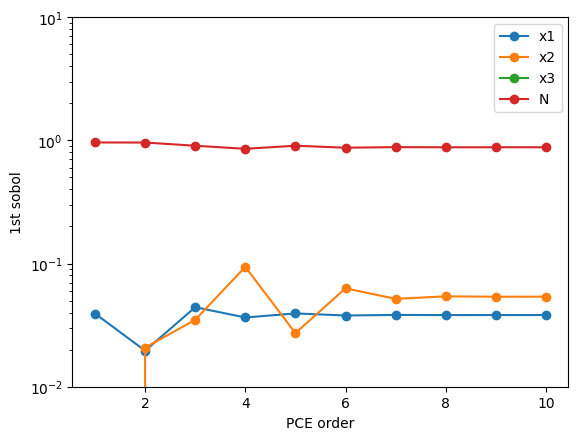
../_images/tutorials_easyvvuq_Ishigami_with_noise_tutorial_12_0.png

[13]:

# plot the first Sobols as a function of PCE order
O = [R[r]['order'] for r in list(R.keys())]
plt.figure()
for v in list(R[O[0]]['results'].sobols_first('Ishigami').keys()):
    plt.semilogy([o for o in O],
                 [R[o]['results'].sobols_first('Ishigami')[v] for o in O],
                 'o-',
                 label=v)
plt.xlabel('PCE order')
plt.ylabel('1st sobol')
plt.ylim(1e-2,10)
plt.legend(loc=0)
plt.savefig('Convergence_sobol_first.png')
plt.savefig('Convergence_sobol_first.pdf')

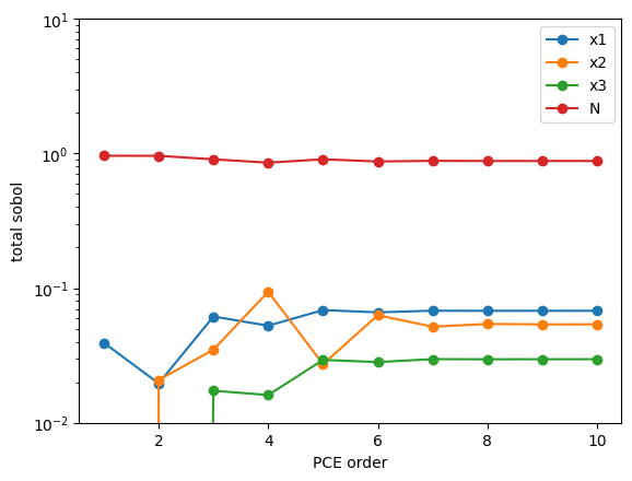
../_images/tutorials_easyvvuq_Ishigami_with_noise_tutorial_13_0.png

[14]:

# plot the total Sobols as a function of PCE order
O = [R[r]['order'] for r in list(R.keys())]
plt.figure()
for v in list(R[O[0]]['results'].sobols_total('Ishigami').keys()):
    plt.semilogy([o for o in O],
                 [R[o]['results'].sobols_total('Ishigami')[v] for o in O],
                 'o-',
                 label=v)
plt.xlabel('PCE order')
plt.ylabel('total sobol')
plt.ylim(1e-2,10)
plt.legend(loc=0)
plt.savefig('Convergence_sobol_total.png')
plt.savefig('Convergence_sobol_total.pdf')

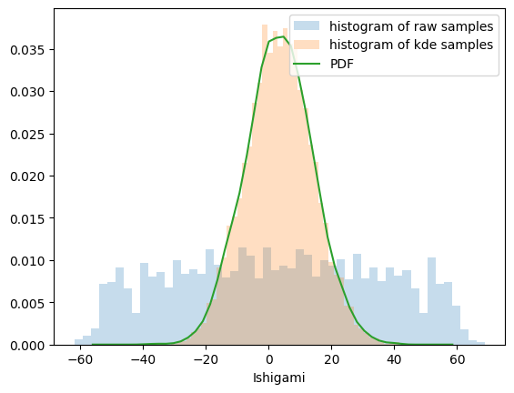
../_images/tutorials_easyvvuq_Ishigami_with_noise_tutorial_14_0.png

[15]:

# plot the distribution function

results_df = R[O[-1]]['results_df']
results = R[O[-1]]['results']
Ishigami_dist = results.raw_data['output_distributions']['Ishigami']

plt.figure()
plt.hist(results_df.Ishigami[0], density=True, bins=50, label='histogram of raw samples', alpha=0.25)
if hasattr(Ishigami_dist, 'samples'):
    plt.hist(Ishigami_dist.samples[0], density=True, bins=50, label='histogram of kde samples', alpha=0.25)
t1 = Ishigami_dist[0]
plt.plot(np.linspace(t1.lower, t1.upper), t1.pdf(np.linspace(t1.lower, t1.upper)), label='PDF')
plt.legend(loc=0)
plt.xlabel('Ishigami')
plt.savefig('Ishigami_distribution_function.png')

../_images/tutorials_easyvvuq_Ishigami_with_noise_tutorial_15_0.png

[16]:

results_df.Ishigami[0]

[16]:

0       -52.525277
1       -40.006931
2       -29.296497
3       -19.405615
4        -9.933955
           ...
14636     9.999347
14637    19.471007
14638    29.361888
14639    40.072323
14640    52.590669
Name: 0, Length: 14641, dtype: float64

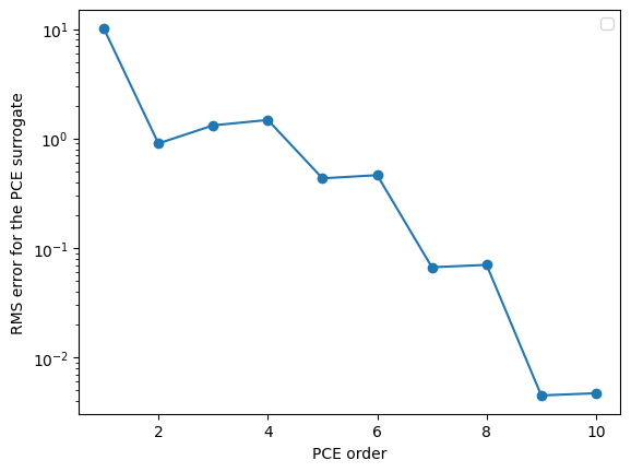
[17]:

# plot the RMS surrogate error at the PCE sample points
_o = []
_RMS = []
for r in R.values():
    results_df = r['results_df']
    results = r['results']
    Ishigami_surrogate = np.squeeze(np.array(results.surrogate()(results_df[results.inputs])['Ishigami']))
    Ishigami_samples = np.squeeze(np.array(results_df['Ishigami']))
    _RMS.append((np.sqrt((((Ishigami_surrogate - Ishigami_samples))**2).mean())))
    _o.append(r['order'])

plt.figure()
plt.semilogy(_o, _RMS, 'o-')
plt.xlabel('PCE order')
plt.ylabel('RMS error for the PCE surrogate')
plt.legend(loc=0)
plt.savefig('Convergence_surrogate.png')
plt.savefig('Convergence_surrogate.pdf')

/var/folders/6f/rn14629n60j16dc99dtk7bs4000ctx/T/ipykernel_79781/2720742683.py:16: UserWarning: No artists with labels found to put in legend.  Note that artists whose label start with an underscore are ignored when legend() is called with no argument.
  plt.legend(loc=0)

../_images/tutorials_easyvvuq_Ishigami_with_noise_tutorial_17_1.png

[18]:

# prepare the test data
test_campaign = uq.Campaign(name='Ishigami.')
test_campaign.add_app(name="Ishigami", params=define_params(),
                      actions=uq.actions.Actions(uq.actions.ExecutePython(run_ishigami_model)))
test_campaign.set_sampler(uq.sampling.quasirandom.LHCSampler(vary=define_vary(), count=100))
test_campaign.execute(nsamples=1000, sequential=True).collate(progress_bar=True)
test_df = test_campaign.get_collation_result()

100%|█████████████████████████████████████| 1000/1000 [00:00<00:00, 6513.72it/s]

[19]:

# calculate the PCE surrogates
test_points = test_df[test_campaign.get_active_sampler().vary.get_keys()]
test_results = np.squeeze(test_df['Ishigami'].values)
test_predictions = {}
for i in list(R.keys()):
    test_predictions[i] = np.squeeze(np.array(R[i]['results'].surrogate()(test_points)['Ishigami']))

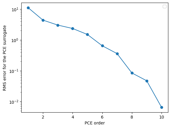
[20]:

# plot the convergence of the surrogate
_o = []
_RMS = []
for r in R.values():
    _RMS.append((np.sqrt((((test_predictions[r['order']] - test_results))**2).mean())))
    _o.append(r['order'])

plt.figure()
plt.semilogy(_o, _RMS, 'o-')
plt.xlabel('PCE order')
plt.ylabel('RMS error for the PCE surrogate')
plt.legend(loc=0)
plt.savefig('Convergence_PCE_surrogate.png')
plt.savefig('Convergence_PCE_surrogate.pdf')

/var/folders/6f/rn14629n60j16dc99dtk7bs4000ctx/T/ipykernel_79781/3799094119.py:12: UserWarning: No artists with labels found to put in legend.  Note that artists whose label start with an underscore are ignored when legend() is called with no argument.
  plt.legend(loc=0)

../_images/tutorials_easyvvuq_Ishigami_with_noise_tutorial_20_1.png

[ ]: