Sensitivity analysis of Ishigami function with Stochastic Collocation

Run an EasyVVUQ campaign to analyze the sensitivity for the Ishigami function

This is done with SC.

[1]:

# Run an EasyVVUQ campaign to analyze the sensitivity for the Ishigami function
# This is done with SC.
%matplotlib inline
import os
import easyvvuq as uq
import chaospy as cp
import pickle
import numpy as np
import matplotlib.pylab as plt
import time
import pandas as pd

[2]:

np.__version__

[2]:

'1.26.4'

[3]:

# Define the Ishigami function
def ishigamiSA(a,b):
    '''Exact sensitivity indices of the Ishigami function for given a and b.
    From https://openturns.github.io/openturns/master/examples/meta_modeling/chaos_ishigami.html
    '''
    var = 1.0/2 + a**2/8 + b*np.pi**4/5 + b**2*np.pi**8/18
    S1 = (1.0/2 + b*np.pi**4/5+b**2*np.pi**8/50)/var
    S2 = (a**2/8)/var
    S3 = 0
    S13 = b**2*np.pi**8/2*(1.0/9-1.0/25)/var
    exact = {
            'expectation' : a/2,
            'variance' : var,
            'S1' : (1.0/2 + b*np.pi**4/5+b**2*np.pi**8.0/50)/var,
            'S2' : (a**2/8)/var,
            'S3' : 0,
            'S12' : 0,
            'S23' : 0,
            'S13' : S13,
            'S123' : 0,
            'ST1' : S1 + S13,
            'ST2' : S2,
            'ST3' : S3 + S13
            }
    return exact

Ishigami_a = 7.0
Ishigami_b = 0.1
exact = ishigamiSA(Ishigami_a, Ishigami_b)

[4]:

# define a model to run the Ishigami code directly from python, expecting a dictionary and returning a dictionary
def run_ishigami_model(input):
    import Ishigami
    qois = ["Ishigami"]
    del input['out_file']
    return {qois[0]: Ishigami.evaluate(**input)}

[5]:

# Define parameter space
def define_params():
    return {
        "x1":       {"type": "float",   "min": -np.pi,     "max": np.pi,      "default": 0.0},
        "x2":       {"type": "float",   "min": -np.pi,     "max": np.pi,      "default": 0.0},
        "x3":       {"type": "float",   "min": -np.pi,     "max": np.pi,      "default": 0.0},
        "a":        {"type": "float",   "min": Ishigami_a, "max": Ishigami_a, "default": Ishigami_a},
        "b":        {"type": "float",   "min": Ishigami_b, "max": Ishigami_b, "default": Ishigami_b},
        "out_file": {"type": "string",  "default": "output.csv"}
    }

[6]:

# Define parameter space
def define_vary():
    return {
        "x1":   cp.Uniform(-np.pi, np.pi),
        "x2":   cp.Uniform(-np.pi, np.pi),
        "x3":   cp.Uniform(-np.pi, np.pi)
    }

[7]:

# Set up and run a campaign
def run_campaign(sc_order=2, use_files=False):

    times = np.zeros(7)

    time_start = time.time()
    time_start_whole = time_start

    # Set up a fresh campaign called "Ishigami_sc."
    my_campaign = uq.Campaign(name='Ishigami_sc.')


    # Create an encoder and decoder for SC test app
    if use_files:
        encoder = uq.encoders.GenericEncoder(template_fname='Ishigami.template',
                                             delimiter='$',
                                             target_filename='Ishigami_in.json')

        decoder = uq.decoders.SimpleCSV(target_filename="output.csv",
                                        output_columns=["Ishigami"])

        execute = uq.actions.ExecuteLocal('python3 %s/Ishigami.py Ishigami_in.json' % (os.getcwd()))

        actions = uq.actions.Actions(uq.actions.CreateRunDirectory('/tmp'),
                          uq.actions.Encode(encoder), execute, uq.actions.Decode(decoder))
    else:
        actions = uq.actions.Actions(uq.actions.ExecutePython(run_ishigami_model))

    # Add the app (automatically set as current app)
    my_campaign.add_app(name="Ishigami", params=define_params(), actions=actions)

    # Create the sampler
    time_end = time.time()
    times[1] = time_end-time_start
    print('Time for phase 1 = %.3f' % (times[1]))

    time_start = time.time()
    # Associate a sampler with the campaign
    my_campaign.set_sampler(uq.sampling.SCSampler(vary=define_vary(), polynomial_order=sc_order))

    # Will draw all (of the finite set of samples)
    my_campaign.draw_samples()
    print('Number of samples = %s' % my_campaign.get_active_sampler().count)

    time_end = time.time()
    times[2] = time_end-time_start
    print('Time for phase 2 = %.3f' % (times[2]))

    time_start = time.time()
    # Run the cases
    my_campaign.execute(sequential=True).collate(progress_bar=True)

    time_end = time.time()
    times[3] = time_end-time_start
    print('Time for phase 3 = %.3f' % (times[3]))

    time_start = time.time()
    # Get the results
    results_df = my_campaign.get_collation_result()

    time_end = time.time()
    times[4] = time_end-time_start
    print('Time for phase 4 = %.3f' % (times[4]))

    time_start = time.time()
    # Post-processing analysis
    results = my_campaign.analyse(qoi_cols=["Ishigami"])

    time_end = time.time()
    times[5] = time_end-time_start
    print('Time for phase 5 = %.3f' % (times[5]))

    time_start = time.time()
    # Save the results
    pickle.dump(results, open('Ishigami_results.pickle','bw'))
    time_end = time.time()
    times[6] = time_end-time_start
    print('Time for phase 6 = %.3f' % (times[6]))

    times[0] = time_end - time_start_whole

    return results_df, results, times, sc_order, my_campaign.get_active_sampler().count

[8]:

# Calculate the stochastic collocation expansion for a range of orders

R = {}
for sc_order in range(1, 21):
    R[sc_order] = {}
    (R[sc_order]['results_df'],
     R[sc_order]['results'],
     R[sc_order]['times'],
     R[sc_order]['order'],
     R[sc_order]['number_of_samples']) = run_campaign(sc_order=sc_order, use_files=False)

Time for phase 1 = 0.047
Number of samples = 8
Time for phase 2 = 0.035

100%|███████████████████████████████████████████| 8/8 [00:00<00:00, 2196.69it/s]

Time for phase 3 = 0.026
Time for phase 4 = 0.004
Time for phase 5 = 0.004
Time for phase 6 = 0.002
Time for phase 1 = 0.007
Number of samples = 27
Time for phase 2 = 0.038

100%|█████████████████████████████████████████| 27/27 [00:00<00:00, 4843.93it/s]

Time for phase 3 = 0.010
Time for phase 4 = 0.002
Time for phase 5 = 0.009
Time for phase 6 = 0.001
Time for phase 1 = 0.006
Number of samples = 64
Time for phase 2 = 0.060


100%|█████████████████████████████████████████| 64/64 [00:00<00:00, 6232.83it/s]

Time for phase 3 = 0.015
Time for phase 4 = 0.002
Time for phase 5 = 0.017
Time for phase 6 = 0.001
Time for phase 1 = 0.005
Number of samples = 125
Time for phase 2 = 0.088

100%|███████████████████████████████████████| 125/125 [00:00<00:00, 6635.80it/s]

Time for phase 3 = 0.024
Time for phase 4 = 0.003
Time for phase 5 = 0.031
Time for phase 6 = 0.001
Time for phase 1 = 0.006
Number of samples = 216
Time for phase 2 = 0.129

100%|███████████████████████████████████████| 216/216 [00:00<00:00, 6528.19it/s]

Time for phase 3 = 0.040
Time for phase 4 = 0.004
Time for phase 5 = 0.053
Time for phase 6 = 0.001
Time for phase 1 = 0.008

Number of samples = 343
Time for phase 2 = 0.183

100%|███████████████████████████████████████| 343/343 [00:00<00:00, 6026.43it/s]

Time for phase 3 = 0.148
Time for phase 4 = 0.005

Time for phase 5 = 0.099
Time for phase 6 = 0.001
Time for phase 1 = 0.006
Number of samples = 512
Time for phase 2 = 0.253

100%|███████████████████████████████████████| 512/512 [00:00<00:00, 5871.77it/s]

Time for phase 3 = 0.101
Time for phase 4 = 0.010

Time for phase 5 = 0.157
Time for phase 6 = 0.002
Time for phase 1 = 0.006
Number of samples = 729
Time for phase 2 = 0.296

100%|███████████████████████████████████████| 729/729 [00:00<00:00, 6839.85it/s]

Time for phase 3 = 0.123
Time for phase 4 = 0.009

Time for phase 5 = 0.234
Time for phase 6 = 0.002
Time for phase 1 = 0.006
Number of samples = 1000
Time for phase 2 = 0.371

100%|█████████████████████████████████████| 1000/1000 [00:00<00:00, 6250.98it/s]

Time for phase 3 = 0.181
Time for phase 4 = 0.011

Time for phase 5 = 0.327
Time for phase 6 = 0.002
Time for phase 1 = 0.018
Number of samples = 1331
Time for phase 2 = 0.510

100%|█████████████████████████████████████| 1331/1331 [00:00<00:00, 6795.01it/s]

Time for phase 3 = 0.223
Time for phase 4 = 0.014
Time for phase 5 = 0.461
Time for phase 6 = 0.005
Time for phase 1 = 0.017
Number of samples = 1728
Time for phase 2 = 0.628

100%|█████████████████████████████████████| 1728/1728 [00:00<00:00, 4753.59it/s]

Time for phase 3 = 0.401
Time for phase 4 = 0.021
Time for phase 5 = 0.710
Time for phase 6 = 0.004
Time for phase 1 = 0.006
Number of samples = 2197
Time for phase 2 = 0.727

100%|█████████████████████████████████████| 2197/2197 [00:00<00:00, 4872.05it/s]

Time for phase 3 = 0.494
Time for phase 4 = 0.022
Time for phase 5 = 0.949
Time for phase 6 = 0.004
Time for phase 1 = 0.006
Number of samples = 2744
Time for phase 2 = 0.849

100%|█████████████████████████████████████| 2744/2744 [00:00<00:00, 6316.13it/s]

Time for phase 3 = 0.559
Time for phase 4 = 0.028
Time for phase 5 = 1.308
Time for phase 6 = 0.005
Time for phase 1 = 0.008
Number of samples = 3375
Time for phase 2 = 1.287

100%|█████████████████████████████████████| 3375/3375 [00:00<00:00, 5507.12it/s]

Time for phase 3 = 0.699
Time for phase 4 = 0.122
Time for phase 5 = 1.867
Time for phase 6 = 0.010
Time for phase 1 = 0.009
Number of samples = 4096
Time for phase 2 = 1.295

100%|█████████████████████████████████████| 4096/4096 [00:00<00:00, 6287.32it/s]

Time for phase 3 = 0.731
Time for phase 4 = 0.114
Time for phase 5 = 2.538
Time for phase 6 = 0.012
Time for phase 1 = 0.011
Number of samples = 4913
Time for phase 2 = 1.524

100%|█████████████████████████████████████| 4913/4913 [00:00<00:00, 5984.61it/s]

Time for phase 3 = 0.915
Time for phase 4 = 0.123
Time for phase 5 = 3.376
Time for phase 6 = 0.423
Time for phase 1 = 0.014
Number of samples = 5832
Time for phase 2 = 1.861

100%|█████████████████████████████████████| 5832/5832 [00:00<00:00, 6221.33it/s]

Time for phase 3 = 1.115
Time for phase 4 = 0.140
Time for phase 5 = 4.407
Time for phase 6 = 0.013
Time for phase 1 = 0.010
Number of samples = 6859
Time for phase 2 = 2.084

100%|█████████████████████████████████████| 6859/6859 [00:01<00:00, 6533.70it/s]

Time for phase 3 = 1.242
Time for phase 4 = 0.135
Time for phase 5 = 5.694
Time for phase 6 = 0.022
Time for phase 1 = 0.011
Number of samples = 8000
Time for phase 2 = 2.377

100%|█████████████████████████████████████| 8000/8000 [00:01<00:00, 6499.63it/s]

Time for phase 3 = 1.378
Time for phase 4 = 0.149
Time for phase 5 = 7.615
Time for phase 6 = 0.023
Time for phase 1 = 0.016
Number of samples = 9261
Time for phase 2 = 2.595

100%|█████████████████████████████████████| 9261/9261 [00:01<00:00, 6123.90it/s]

Time for phase 3 = 1.746
Time for phase 4 = 0.167
Time for phase 5 = 14.192
Time for phase 6 = 0.023

[9]:

# save the results

pickle.dump(R, open('collected_results.pickle','bw'))

[10]:

# produce a table of the time taken for various phases
# the phases are:
#   1: creation of campaign
#   2: creation of samples
#   3: running the cases
#   4: calculation of statistics including Sobols
#   5: returning of analysed results
#   6: saving campaign and pickled results

Timings = pd.DataFrame(np.array([R[r]['times'] for r in list(R.keys())]),
             columns=['Total', 'Phase 1', 'Phase 2', 'Phase 3', 'Phase 4', 'Phase 5', 'Phase 6'],
             index=[R[r]['order'] for r in list(R.keys())])
Timings.to_csv(open('Timings.csv', 'w'))
display(Timings)

	Total	Phase 1	Phase 2	Phase 3	Phase 4	Phase 5	Phase 6
1	0.116857	0.046528	0.034933	0.025752	0.003636	0.004290	0.001542
2	0.066798	0.006985	0.038313	0.009610	0.001932	0.009117	0.000763
3	0.100764	0.005955	0.060359	0.014736	0.002238	0.016597	0.000803
4	0.151393	0.005356	0.087646	0.023992	0.002885	0.030742	0.000696
5	0.234107	0.005735	0.129114	0.040493	0.004272	0.053385	0.001017
6	0.445746	0.008459	0.183465	0.148184	0.005055	0.098970	0.001456
7	0.528847	0.005818	0.253195	0.101443	0.009872	0.156532	0.001785
8	0.668787	0.005989	0.295620	0.122671	0.008789	0.233810	0.001744
9	0.898134	0.006197	0.370832	0.181402	0.010727	0.326783	0.002029
10	1.231645	0.017721	0.510358	0.223078	0.014288	0.460788	0.005255
11	1.781211	0.017318	0.628123	0.400859	0.021470	0.709611	0.003593
12	2.202862	0.005997	0.727173	0.493930	0.022408	0.948569	0.004500
13	2.756144	0.006344	0.848810	0.559102	0.027787	1.308449	0.005416
14	3.993149	0.007872	1.286562	0.699052	0.121875	1.866614	0.010422
15	4.700541	0.009332	1.295280	0.731292	0.113867	2.538433	0.011786
16	6.373810	0.010733	1.524221	0.915396	0.123134	3.376400	0.423174
17	7.550553	0.014175	1.860752	1.115186	0.139940	4.407107	0.012942
18	9.188759	0.009911	2.084367	1.242440	0.135266	5.694486	0.021989
19	11.553041	0.011360	2.376985	1.377563	0.148670	7.614944	0.022871
20	18.739314	0.016116	2.594794	1.746175	0.167113	14.191557	0.022820

[11]:

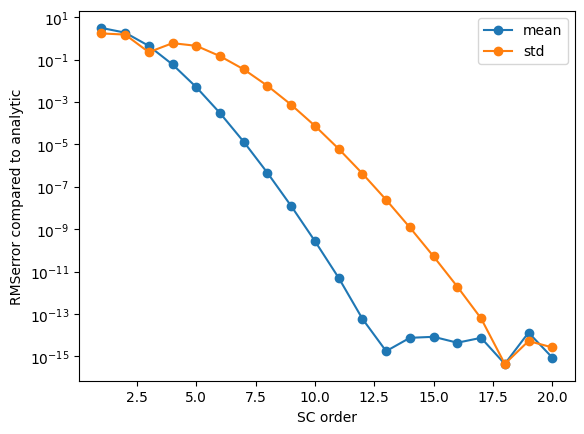
# plot the convergence of the mean and standard deviation to that of the highest order

mean_analytic = exact['expectation']
std_analytic = np.sqrt(exact['variance'])

O = [R[r]['order'] for r in list(R.keys())]
plt.figure()
plt.semilogy([o for o in O],
             [np.abs(R[o]['results'].describe('Ishigami', 'mean') - mean_analytic) for o in O],
             'o-', label='mean')
plt.semilogy([o for o in O],
             [np.abs(R[o]['results'].describe('Ishigami', 'std') - std_analytic) for o in O],
             'o-', label='std')
plt.xlabel('SC order')
plt.ylabel('RMSerror compared to analytic')
plt.legend(loc=0)
plt.savefig('Convergence_mean_std.png')
plt.savefig('Convergence_mean_std.pdf')

../_images/tutorials_easyvvuq_Ishigami_SC_tutorial_12_0.png

[12]:

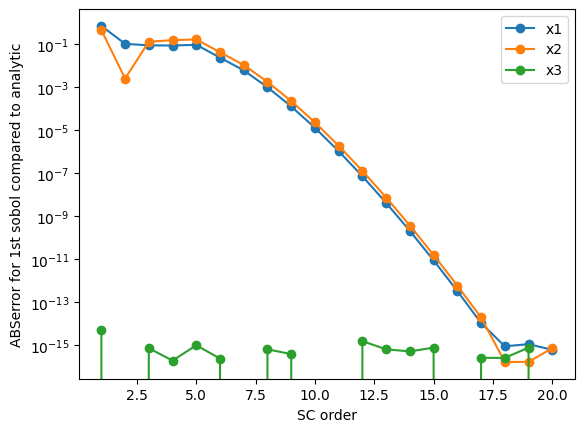
# plot the convergence of the first sobol to that of the highest order

sobol_first_exact = {'x1': exact['S1'], 'x2': exact['S2'], 'x3': exact['S3']}

O = [R[r]['order'] for r in list(R.keys())]
plt.figure()
for v in list(R[O[0]]['results'].sobols_first('Ishigami').keys()):
    plt.semilogy([o for o in O],
                 [np.abs(R[o]['results'].sobols_first('Ishigami')[v] - sobol_first_exact[v]) for o in O],
                 'o-',
                 label=v)
plt.xlabel('SC order')
plt.ylabel('ABSerror for 1st sobol compared to analytic')
plt.legend(loc=0)
plt.savefig('Convergence_sobol_first.png')
plt.savefig('Convergence_sobol_first.pdf')

../_images/tutorials_easyvvuq_Ishigami_SC_tutorial_13_0.png

[13]:

# prepare the test data
test_campaign = uq.Campaign(name='Ishigami.')
test_campaign.add_app(name="Ishigami", params=define_params(),
                      actions=uq.actions.Actions(uq.actions.ExecutePython(run_ishigami_model)))
test_campaign.set_sampler(uq.sampling.quasirandom.LHCSampler(vary=define_vary(), count=100))
test_campaign.execute(nsamples=1000, sequential=True).collate(progress_bar=True)
test_df = test_campaign.get_collation_result()

100%|█████████████████████████████████████| 1000/1000 [00:00<00:00, 6667.73it/s]

[14]:

# calculate the SC surrogates
if __name__ == '__main__':

    test_points = test_df[test_campaign.get_active_sampler().vary.get_keys()]
    test_results = np.squeeze(test_df['Ishigami'].values)
    test_predictions = {}
    for i in list(R.keys()):
        test_predictions[i] = np.squeeze(np.array(R[i]['results'].surrogate()(test_points)['Ishigami']))

[15]:

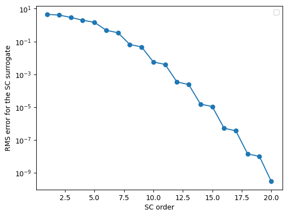
# plot the convergence of the surrogate
if __name__ == '__main__':
    _o = []
    _RMS = []
    for r in R.values():
        _RMS.append((np.sqrt((((test_predictions[r['order']] - test_results))**2).mean())))
        _o.append(r['order'])

    plt.figure()
    plt.semilogy(_o, _RMS, 'o-')
    plt.xlabel('SC order')
    plt.ylabel('RMS error for the SC surrogate')
    plt.legend(loc=0)
    plt.savefig('Convergence_SC_surrogate.png')
    plt.savefig('Convergence_SC_surrogate.pdf')

/var/folders/6f/rn14629n60j16dc99dtk7bs4000ctx/T/ipykernel_67300/2228134460.py:13: UserWarning: No artists with labels found to put in legend.  Note that artists whose label start with an underscore are ignored when legend() is called with no argument.
  plt.legend(loc=0)

../_images/tutorials_easyvvuq_Ishigami_SC_tutorial_16_1.png

[ ]: